

![]()
%matplotlib inline
from matplotlib.pyplot import *
from numpy import *  ## for numerical functions
from IPython.display import Audio  ## to output audio
Mathematics of Sound
What is sound?
Rapid changes, or vibrations in air pressure are heard in our ears as sound.
A computer creates sound by sending a list of numbers to a speaker, which then vibrates.
Random numbers
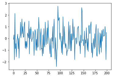
A list of random numbers, will create a sound.
What do you think 44,000 random numbers will sound like?
Fs = 44100
random_sd = random.randn(Fs)
## Random sound
Audio(data=random_sd, rate=Fs)
We can plot a few of those numbers, using a plotting command.
plot(random_sd[0:200]);
Periodic vibrations
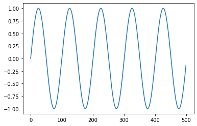
A vibration that has a periodic vibration will sound like a tone to us.
The sine function has a periodic cycle, and can be used to represent such a tone.
Fs, Len, f1 = 44100, 3, 440  ## sample rate, length in seconds, frequency
t = linspace(0,Len,Fs*Len)  ## time variable
sine_sd = sin(2*pi*440*t)
Audio(data=sine_sd, rate=Fs)
We can plot this sine sound, using a plotting command.
plot(sine_sd[0:500]);
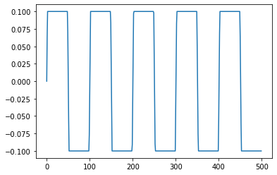
By clipping the tops of the sine wave, we get a square wave.
square_sd = minimum(.1, maximum(-.1,sine_sd))
plot(square_sd[0:500]);
## What does a square wave sound like?
Audio(data=square_sd, rate=Fs)
The Sine and Square waves have the same pitch (frequency) but different timbres.
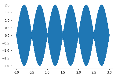
Beats
Playing two tones at similar frequencies results in beats. This is useful for tuning instruments!
sine2_sd = sin(2*pi*440*t) - sin(2*pi*442*t)
Audio(data=sine2_sd, rate=Fs)
We can plot to see the beats, or variations in amplitude.
Note we plot the whole 3 seconds of the sound. Two beats per second.
plot(t,sine2_sd);
A chirp
Bats use chirps, tones that rapidly increase in frequency, for echolocation like sonar.
We can use a chirp to explore the range of frequencies that we can hear.
Humans (with very good ears) can hear from 20 Hz to 20,000 Hz.
f = 20000/(2*Len)
chirp_sd = sin(2*pi*f*t**2) ## t**2 creates the increasing freq's.

Audio(data=chirp_sd, rate=Fs)
Count the pulses
We test how well you hear, by testing various frequencies.
freq = 10000

n = random.randint(1,5)
test_sd = sin(2*pi*freq*t)*sin(pi*n*t/Len)
Audio(data=test_sd,rate=Fs,autoplay=True)
More on chirps.
We can vary the parameters, to vary the sounds
Fs = 44100
Len = 3
t = linspace(0,Len,Fs*Len)
fmax = 15000
chirp2_sd = sin(pi*(fmax/Len)*t**2)

Audio(data=chirp2_sd, rate=Fs,autoplay=True)
Summary
This notebook was a brief introduction to the mathematics of sound. We generated vibrations in air pressure using code that the computer sent to speakers.
We learned about sine and square waves, beats, and chirps.
For more information on these topics, check out the notebook on the mathematics of pitch.
