Bubonic Plage - SIR Model¶

The SIR Outbreak Model¶

Population Parameters¶

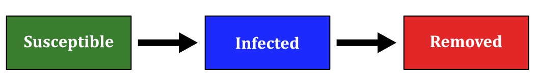
In this model, the total population is divided into three groups:

Susceptible: individuals that can become infected but haven’t been yet
Infected: individuals that are infected
Removed: individuals that are either dead or recovered

We are looking at the changes, over the course of an outbreak, of the numbers of these individuals, represented by $S$, $I$, and $R$. In other words we want to understand how, as time passes, the number of individuals in each group changes.

Having a realistic model might be useful for predicting the long-term outcome of an outbreak and informing public health interventions.

If we can predict that the number of removed people will stay low and the number of infected people will quickly go down to zero, then there is no need to intervene and we can let the outbreak end by itself while only providing medical attention to the infected people.

Conversely if we predict a large increase of the numbers of infected and removed individuals, then the outbreak needs a quick intervention before it results in a large number of casualties. In a plague outbreak this intervention would, for example, be to make sure there is no contact between infected and susceptible people.

We now describe the SIR (Susceptible, Infected, Removed) mathematical model of an outbreak over time (for example every week). We write $S_t, I_t, R_t$ to denote the number of susceptible, infected, and removed individuals at time point $t$. $t=1$ is the first recorded time point, $t=2$ is the second and so on. We call time unit the time elapsed between two time points, for example a day or a week.

In this model, we assume that the total population is constant (so births and deaths are ignored) for the duration of the model simulation. We represent the total population size by $N$, and so at any time point $t$ we have $$N=S_t + I_t + R_t$$

Modelling the disease progression¶

We assume that transmission requires contact between an infected individual and a susceptible individual. We also assume that the disease takes a constant amount of time to progress within an infected individual until they are removed (die or recover). We need to define these two processes (infection and removal) and model how they impact the transition from the time $t = (S_t,I_t,R_t)$ to the next state $t + 1 = (S_{t+1},I_{t+1},R_{t+1})$.

SIR_1

The occurrences of new infections of is modelled using a parameter $\beta$, that gives the proportion of contacts between susceptible people and infected people, during one time unit, that results in infection. Then we can describe the number of newly infected people as $\dfrac{\beta S_t I_t}{N}$, where the term $S_t I_t$ represents the set of all possible contacts between susceptible and infected individuals. We discuss this term later.

The occurrence of removals of infected people is modelled using a parameter denoted by $\gamma$. It is defined to be proportion of infected individuals that die or recover between two time points. If we are given that the duration of an infection is $T$ (i.e. how many time points it takes for an individual between infection and removal), then $\gamma = \dfrac{1}{T}$.

SIR_2

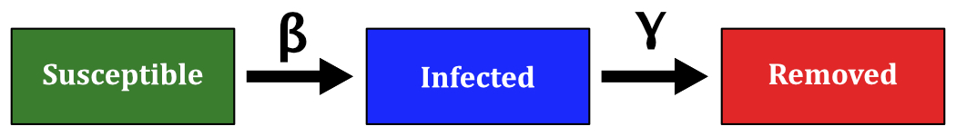
Taking into account the rate of contact $\beta$ and rate of removal $\gamma$, then each group population changes within one unit of time as follows

\[\begin{split} \begin{align} S_{t+1} &= S_t - \dfrac{{\beta} S_t I_t}{N}\\ I_{t+1} &= I_t + \dfrac{{\beta} S_t I_t}{N} - \gamma I_t \\ R_{t+1} &= R_t + \gamma I_t\\ N&=S_t + I_t + R_t \end{align} \end{split}\]

These equations form the SIR model. They allow, from knowing the parameters of the model ($\beta$ and $\gamma$) and the current state ($S_t,I_t,R_t$) of a population to predict the next states of the population for later time points. Such models are critical in our days for monitoring and controlling infectious diseases outbreaks.

Technical remarks.¶

First, note that the SIR model does not enforce that the values $S_t,I_t,R_t$ at a given time point are integers. As $\beta$ and $\gamma$ are actually floating numbers, these values are actually most of the time not integers. This is fine as the SIR model is an approximate model and aims mostly at predicting the general dynamics of an outbreak, not the precise values for the number of susceptible, infected, and removed individuals.

Next, one can ask how to find the values of the parameters $\beta$ and $\gamma$ that are necessary to have a full SIR model.

As discussed above, the parameter $\gamma$ is relatively easy to find from knowing how the disease progress in a patient, as it is mostly the inverse of the average time a patient is sick.

The parameter $\beta$ is less easy to obtain. Reading the equations we can see that during a time point, out of the $S_t$ susceptible individuals, the number that get infected is $(\dfrac{{\beta}}{N}) S_t I_t$. As mentioned above, the product $S_t I_t$ can be interpreted as the set of all possible contacts between the $S_t$ susceptible individuals and the $I_t$ infected individuals and is often a large number, much larger than $S_t$ and in the order of $N^2$. The division by $N$ aims to lower this number, mostly to normalize it by the total population, to make sure it is in order of $N$ and not quadratic in $N$. So in order for the number of newly infected individuals during a time unit to be reasonable, $\beta$ is generally a small number between $0$ and $1$. But formally, if we pick a value for $\beta$ that is too large, then the SIR model will predict value for $S_t$ that can be negative, which is inconsistent with the modelled phenomenon. So choosing the value of $\beta$ is the crucial step in modelling an outbreak.

# This function takes as input a vector y holding all initial values,
#    t: the number of time points (e.g. days)
#    beta: proportion of contacts that result in infections
#    gamma: proportion of infected that are removed
#    S1,I1,R1 = initial population sizes

def discrete_SIR(S1,I1,R1,t,beta,gamma):
    # Empy arrays for each class
    S = [] # susceptible population
    I = [] # infected population
    R = [] # removed population
    N = S1+I1+R1 # the total population
    
    # Append initial values
    S.append(S1)
    I.append(I1)
    R.append(R1)
    
    # apply SIR model: iterate over the total number of days - 1
    for i in range(t-1):
        S_next = S[i] - (beta/N)*((S[i]*I[i]))
        S.append(S_next)
        
        I_next = I[i] + (beta/N)*((S[i]*I[i])) - gamma*I[i]
        I.append(I_next)
        
        R_next = R[i] + gamma * I[i]
        R.append(R_next)
    
    # return arrays S,I,R whose entries are various values for susceptible, infected, removed 
    return((S,I,R))

Modelling an outbreak related to the Great Plague of London¶

The last major epidemic of the bubonic plague in England occurred between 1665 and 1666 (click here for further reading). This epidemic did not kill as many people as the Black Death (1347 - 1351), however it is remembered as the “Great Plague of London” as it was the last widespread outbreak that affected England.

“City records indicate that some 68,596 people died during the epidemic, though the actual number of deaths is suspected to have exceeded 100,000 out of a total population estimated at 460,000. ” Great Plague of London”; Encyclopædia Britannica; Encyclopædia Britannica, inc.; September 08, 2016

When the bubonic plague outbreak hit London, people started to leave the city and go to the countryside, hoping to avoid the disease. But as can be expected, some of these people were already infected when they left London, and so carried the disease to start other outbreaks in some nearby villages. This happened in the village of Eyam.

When Eyam authorities realized a plague outbreak had started, they took the difficult decision to close the village in order to avoid to spread the disease further. So nobody was allowed to enter or leave the village and people stayed there hoping the outbreak would end by itself without too many casualties; note that from a mathematical point of view, that implies that the assumption that the sum of the numbers of susceptible, infected and removed individuals, the population, is constant.

Also the village authorities recorded regularly the number of infected and dead people; these data are described in the table below, for the period from June 19 1665 to October 19 1665, with data being recorded every 2 weeks. Obviously these data are imperfect (some people did not declare they were sick by fear of being ostracized, some people died too fast for the plague to be diagnosed, etc.), but nevertheless, they provide us with interesting data to see if the SIR model is an appropriate model for such a plague outbreak.

| Date |Day Number |Susceptible | Infected | |——-||————-|———-| |June 19 1665|0|254|7| |July 3 1665|14|235|14| |July 19 1665|28|201|22| |Aug 3 1665|42|153|29| |Aug 19 1665|56|121| 21| |Sept 3 1665|70|108|8| |Sept 19 1665|84|121|21| |Oct 3 1665| 98|NA | NA| |Oct 19 1665|112| 83 | 0|

The average time an infected individual remains infected by the bubonic plague is 11 days.

With the information above, we will be able to get the parameters of the SIR model for this outbreak and observe if indeed what this model predicts generates results corresponding to what happened in reality.

Question 1:¶

Assuming that on June 19 no individuals had died, i.e. no one was in the Removed class, what is the value of $N$, i.e. the number of individuals in the total population?

Question 2:¶

We know that the average time an individual remained infected is 11 days. What is the rate of removal ($\gamma$)?

Question 3:¶

We are now trying something more difficult but more interesting. We introduced a mathematical model for outbreaks, but nothing so far shows that this SIR model is appropriate to model an outbreak such as the Eyam plague outbreak. We want to answer this question now.

From questions 1 and 2 above we know the values of $N$ and $\gamma$ (check your answers at the bottom of this notebook). From the data table we also know $S_1,I_1,R_1$, the state of the population at the start of the outbreak. So if we want to apply the SIR model we need to find a value for $\beta$ the parameter, the number susceptible people becoming infected during a time unit. We consider here that a time unit is 1 day; the Eyam outbreak spanned 112 days, so 112 time units, even if data were only recorded every 2 weeks.

A standard scientific approach for the problem of finding $\beta$ is to try various values and see if there is one that leads to predicted values for $S_n,I_n,R_n$ that match the observed data. In order to evaluate this match, we focus on the number of infected people, the most important element of an outbreak.

The code below allows you to do this: you can choose a value of $\beta$, click on the “Run interact” button and it will show on the same graph a set of 8 blue dots (the observed number of infected people from the data table) and a set of 112 red dots, corresponding to the predicted number of infected individuals for the chosen value of $\beta$.

While there are several mathematical ways to define what would be the best fit, here we are not getting into this and you are just asked to try to find a value of $\beta$ that generated blue dots being approximately on the graph defined by the red dots. Pay particular attention to the first four blue dots.

Note that in this case $0 < \beta < 1$.

Warning:¶

The SIR model is a very simple approximation of the dynamics of a true outbreak, so don’t expect to find a value of $\beta$ that generates a graph that contains exactly all observed data points (blue dots).

In particular note that the data from September 3 and 19 seem to be somewhat of an anomaly as we observe a sharp decrease in the number of infected followed by a surge. This could be due to many reasons, for example poor statistics recording (we are considering a group of people under heavy stress likely more motivated by trying to stay alive than to record accurate vital statistics).

So here we are interested in finding a parameter $\beta$ that captures the general dynamics (increase followed by a post-peak decrease) of the outbreak. You can expect to find a reasonable value for $\beta$ but be aware that many values, especially too high, will result in a very poor match between observed data and model predictions.

from ipywidgets import interact_manual, interact,widgets
import matplotlib.pyplot as plt

# set style
s = {'description_width': 'initial'}

# Set interact manual box widget for beta
@interact(answer=widgets.FloatText(value=0.50, description='Enter beta ',
    disabled=False, style=s, step=0.01
))

# define function to find the appropriate value of beta
# this function takes as input a floating value and outputs a plot with the best fit curve
def find_beta(answer):
    
    # set initial values for SIR model
    S1,I1,R1 = 254,7,0
    
    # Use original data on Number of infected from table in the notebook
    ori_data = [7,14,22,29,21,8,21,0]
    
    # use days, time data was provided biweekly, we transform to days here
    ori_days = [1,14,28,42,56,70,84,112]
    
    # set number of days as the second to last entry on the ori_days array 
    n = ori_days[len(ori_days)-1]-ori_days[0]+1
    
    # get beta from answer - to be sure transform to float
    beta = float(answer)
    
    # Gamma was obtained from disease
    gamma = 1/11
    
    # Compute SIR values using our discrete_SIR function
    (S,I,R) = discrete_SIR(S1,I1,R1,n,beta,gamma)
    
    # Figure
    #fig,ax = plt.subplot(figsize=(10,10))
    fig = plt.figure(facecolor='w',figsize=(17,5))
    ax  = fig.add_subplot(111,facecolor = '#ffffff')
    # Scatter plot of original number of infected in the course of 112 days
    
    plt.scatter(ori_days,ori_data,c="blue", label="Original Data")
    
    # Scatter plot of infected obtained from SIR mode, in the course of 112 days
    plt.scatter(range(n),I,c="red",label="SIR Model Predictions")
    
    # Make the plot pretty
    plt.xlabel('Time (days)')
    plt.ylabel('Infected Individuals')
    plt.title('Real Data vs Model')
    #legend = ax.legend()
    plt.show()
    

Simulating a Disease Outbreak¶

To conclude we will use the widgets below to simulate a disease outbreak using the SIR model. You can choose the values of all the elements of the model (sizes of the compartments of the population at the beginning of the outbreak, parameters $\gamma$ and $\beta$, and duration in time units (days) of the outbreak. The default parameters are the ones from the Eyam plague outbreak.

The result is a series of three graphs that shows how the three components of the population change during the outbreak. It allows you to see the impact of changes in the parameters $\gamma$ and $\beta$, such as increasing $\beta$ (making the outbreak progress faster) or reducing $\gamma$ (decreasing the removal rate).

You can use this interactive tool to try to fit the SIR model to match the observed data.

import matplotlib.pyplot as plt
import numpy as np
from math import ceil

# This function takes as input initial values of susceptible, infected and removed, number of days, beta and gamma
# it plots the SIR model with the above conditions
def plot_SIR(S1,I1,R1,n,beta,gamma):
    
    # Initialize figure
    fig = plt.figure(facecolor='w',figsize=(17,5))
    ax  = fig.add_subplot(111,facecolor = '#ffffff')
    
    # Compute SIR values for our initial data and parameters
    (S_f,I_f,R_f) = discrete_SIR(S1,I1,R1,n,beta,gamma)    
    
    # Set x axis
    x = [i for i in range(n)]
   
    # Scatter plot of evolution of susceptible over the course of x days
    plt.scatter(x,S_f,c= 'b',label='Susceptible')
    
    # Scatter plot of evolution of infected over the course of x days
    plt.scatter(x,I_f,c='r',label='Infected')
    
    # Scatter plot of evolution of removed over the course of x days
    plt.scatter(x,R_f,c='g',label='Removed')

    # Make the plot pretty
    plt.xlabel('Time (days)')
    plt.ylabel('Number of individuals')
    plt.title('Simulation of a Disease Outbreak Using the SIR Model')
    legend = ax.legend()
    plt.show()
    
    # Print messages to aid student understand and interpret what is happening in the plot
    print("SIMULATION DATA\n")
    print("Beta: " + str(beta))
    print("Gamma: " + str(gamma))
    print("\n")
    print("Initial Conditions:")
    print("Total number of Susceptible: "  + str(ceil(S_f[0])))
    print("Total number of Infected: "  + str(ceil(I_f[0])))
    print("Total number of Removed: "  + str(ceil(R_f[0])))
    print("\n")
    print("After " + str(n) + " days:")
    print("Total number of Susceptible: "  + str(ceil(S_f[n-1])))
    print("Total number of Infected: "  + str(ceil(I_f[n-1])) )
    print("Total number of Removed: "  + str(ceil(R_f[n-1])))

# Tweaking initial Values
from ipywidgets import widgets, interact, interact_manual

# Set function above so that the user can set all parameters and manually start simulation
s = {'description_width': 'initial'}
interact(plot_SIR,
        S1 = widgets.IntSlider(value=254, min=200, max=1000, step=1, style=s, description="Susceptible Initial", 
                               disabled=False, orientation='horizontal', readout=True),
        I1 = widgets.IntSlider(value=7, min=0, max=500, step=1, style=s, description="Infected Initial",
                               disabled=False, orientation='horizontal', readout=True),
        R1 = widgets.IntSlider(value=0, min=0, max=500, step=1, style=s, description="Removed Initial",
                               disabled=False, orientation='horizontal', readout=True),
        n = widgets.IntSlider(value=112, min=0, max=500, step=1, style=s, description="Time (days)",
                              disabled=False, orientation='horizontal', readout=True),
        beta = widgets.FloatText(value=1.50, description=r'$ \beta$ parameter',
                                 disabled=False, style = s, step=0.01),
        gamma = widgets.FloatText(value=1.50, description= r'$ \gamma$ parameter',
                                  disabled=False, style=s, step=0.01)
        );

Answer 1¶

Since we are assuming the population is constant, and since $S_1 = 254, I_1 = 7, R_1 = 0$, then $S_1 + I_1 + R_1 = 254 + 7 + 0 = 261$.

Answer 2¶

We know that, on average, an individual will remain infected for approximately 11 days. This means that one individual moves to the removed class for every 11 days, and the rate of removal is $\gamma = \frac{1}{11} = 0.0909...$.

Answer 3¶

The best value is approximately $\beta = 0.14909440503418078$.

Conclusion

In this notebook we learned about the SIR discrete model to model an outbreak. We learned that this model is one of the simplest ones and that it separates the total population $N$ (a constant) into three categories: Infected, Susceptible and Removed. We learned about rates of infection and removal and how this affects the number of individuals in each class.

We also ran a basic but realistic simulation of a bubonic plague outbreak of the Great Plague of London that took place in the village Eyam in 1665 and learned about the devastating effect this had on the population.

Callysto Curriculum Notebooks