

![]()
3D Plotting with matplotlib
Matplotlib is a rich collection of commands to create mathematical plots in a Jupyter notebook. It is best to search online for extensive examples.
In this notebook, we will show a few examples on how to do 3D graphs. The basic idea is to set up some data for variables x,y,z, then let the computer plot this into a surface in 3D.
We first import some useful tools from matplotlib:
%matplotlib inline
from mpl_toolkits.mplot3d import Axes3D
from matplotlib.pyplot import *
from numpy import *
Example 1. A simple 3D plot
We will plot a hyperboloid which comes from the quadratic equation \($z = x^2 - y^2.\)$
The key idea is to define a range of values for variables x and y, combine them as a “meshgrid” which is just an array of values, then evaluate the quadratic above to give the z values.
From this data, we then create the 3D figure and plot.
# Make data.
X = [-2,-1,0,1,2]
Y = [-2,-1,0,1,2]
X, Y = meshgrid(X, Y)
Z = X**2 - Y**2

# create the 3D figure
fig = figure()
ax = fig.gca(projection='3d')


# Plot the surface.
surf = ax.plot_surface(X, Y, Z,
                       linewidth=0, antialiased=False)

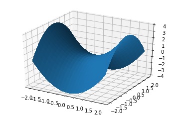
Example 2. A better 3D plot
Let’s plot the same hyperboloid \($z = x^2 - y^2\)$ but with a smoother surface.
The key idea is enrich the range of values for variables x and y, combine them as a “meshgrid” which is just an array of values, then evaluate the quadratic above to give the z values. We use the numpy function “linspace” to get more data points into the picture.
From this data, we then create the 3D figure and plot.
# Make data.
X = linspace(-2,2,25)
Y = linspace(-2,2,25)
X, Y = meshgrid(X, Y)
Z = X**2 - Y**2

# create the 3D figure
fig = figure()
ax = fig.gca(projection='3d')


# Plot the surface.
surf = ax.plot_surface(X, Y, Z,
                       linewidth=0, antialiased=False)
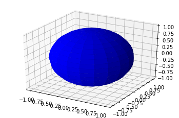
Example 3. A parametric 3D plot
We can also plot parametrized surfaces. For instance, a sphere of radius one can be defined in parametric form as \($ \begin{eqnarray} x & = & \cos(u)\sin(v) \\ y & = & \sin(u)\sin(v) \\ x & = & \cos(v) \end{eqnarray} $\) where \(u\in[0,2\pi]\) is the azimuthal angle and \(v\in[0,\pi]\) is the polar angle.
The “outer” function from numpy gives a fast way to compute the products of these functions of u and v.
# Make data
u = linspace(0, 2 * pi, 20)
v = linspace(0, pi, 20)
x = outer(cos(u), sin(v))
y = outer(sin(u), sin(v))
z = outer(ones(size(u)), cos(v))

## Create a 3D figure
fig = figure()
ax = fig.add_subplot(111, projection='3d')

# Plot the surface
ax.plot_surface(x, y, z, color='b')

show()
More examples
More information on 3D plotting here: https://matplotlib.org/mpl_toolkits/mplot3d/tutorial.html
