

![]()
from IPython.display import HTML
from IPython.display import display, Math, Latex
import numpy as np
import matplotlib.pyplot as plt
import ipywidgets as widgets

HTML('''<script>
  function code_toggle() {
    if (code_shown){
      $('div.input').hide();
      $('#toggleButton').val('Show Code')
    } else {
      $('div.input').show();
      $('#toggleButton').val('Hide Code')
    }
    code_shown = !code_shown
  }

  $( document ).ready(function(){
    code_shown=false;
    $('div.input').hide()
  });
</script>
<form action="javascript:code_toggle()"><input type="submit" id="toggleButton" value="Show Code"></form''')
Half life calculations
Radioactive elements decay in an unpredictable way. There is no way to tell whether the nucleus of uranium will decay by the time you finish reading this sentence, or after lunch, or in 100 years. However, it is possible to predict how many nuclei in a sample will decay in a given time.
In this notebook, we will look at solving questions about radioactive decay using the concept of the half-life, without the use of logarithms.
Half-life
The half-life of an element is the time required for one half of a radioactive element to decay into something else (either by alpha, beta, or gamma decay. A common symbol for half-life is \(t_{1/2}\). It’s important to note that that total sample doesn’t decay by 50% every half-life - 50% of the remaining radioactive substance decays every half-life. For example, if we initially have 100 grams of a radioactive material with a half life of one year, after the first year there will be 50 grams of the radioactive substance left (and 50 grams of its stable daughter element). After two years, there will be 25 grams remaining (and 75 grams of the daughter element) etc. We can see this idea visualized in the gif in the introduction of this notebook.
Radioactive Decay Equation and Curves
The rate at which a sample decays depends on how much radioactive material is present. As more of the radioactive sample decays, the probability of more decaying becomes smaller, and the rate at which it decays slows down; the decay rate (or activity, A) is proportional to the number of radioactive atoms, N:
This type of relationship results in an exponential decay of the sample. If we have an initial number (\(N_0\)) of radioactive nuclei with half-life \(t_{1/2}\), the number of nuclei remaining (\(N\)) after a time \(t\) is given by the equation:
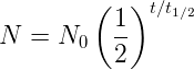
Below is the plot of a radiation curve of an imaginary element with a half-life of 4 days.
def N(N_0,x,t_hl):
    return N_0 * (1/2) ** (x/t_hl)

x = np.linspace(0,20,1000)
plt.figure(figsize=(11,8),num = "fig 1")
plt.plot(x,N(4,x,4), linewidth=2)
plt.title('Radioactive Decay Curve', fontsize=20)
plt.xlabel('Time (days)', fontsize=18)
plt.ylabel('Amount of element remaining (grams)', fontsize=18)
plt.xticks(np.arange(min(x), max(x)+1, 1.0))
plt.xticks(fontsize=15)
plt.yticks(fontsize=15)
plt.xlim([0,20])
plt.ylim([0,4])
plt.grid(alpha=0.8, linestyle='--')
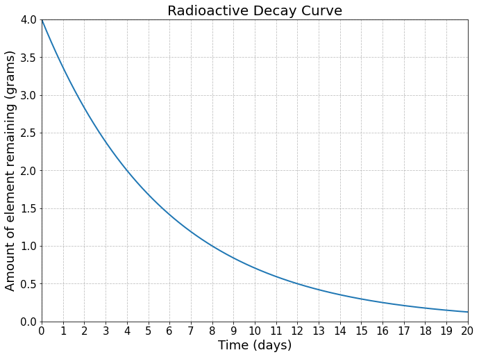
We can tell the half-life of the element from the graph quite easily. At time \(t=0\), we initially have 4 grams of the substance. After a time of \(t_{1/2}\) passes, half of the substance will decay, so there will be 2 grams left. From the graph, we can see that there are 2 grams eft after exactly 4 days. Thus, for this element, \(t_{1/2} = 4\) days.
Below we will present some more radiation curves. Try to determine the half-life of the element, just as we did here. To check if your answer is correct, press the Enter key after you type your answer in each text box.
file = open("images/iodine-131.png","rb")
image = file.read()
plot = widgets.Image(value=image, format='png', width=775,height=1150)
display(plot)

counter11=0
t1 = widgets.Text(placeholder="Enter the half-life here")

def callback(b):
    global counter11
    counter11 += 1
    if counter11 < 4:
        answer = t1.value.replace(" ", "").lower()
        if answer == "8days":
            display(Latex("Excellent, that's correct!"))
            counter11=5
        else:
            display(Latex("Not quite - try again! Hint: Make sure you inclued the units! Ex. _ seconds"))
    elif counter11 == 4:
        display(Latex("The half-life is 8 days"))

t1.on_submit(callback)
display(t1)
file = open("images/caesium-137.png","rb")
image = file.read()
plot = widgets.Image(value=image, format='png', width=775,height=1150,)
display(plot)

counter12=0
t2 = widgets.Text(placeholder= "Enter the half-life here")

def callback(b):
    global counter12
    counter12 += 1
    if counter12 < 4:
        answer = t2.value.replace(" ", "").lower()
        if answer == "30years":
            display(Latex("Excellent, that's correct!"))
            counter12=5
        else:
            display(Latex("Not quite - try again! Hint: Make sure you inclued the units! Ex. _ seconds"))
    elif counter12 == 4:
        display(Latex("The half-life is 30 years"))

t2.on_submit(callback)
display(t2)
file = open("images/curium-245.png","rb")
image = file.read()
plot = widgets.Image(value=image, format='png', width=775,height=1150,)
display(plot)

counter13=0
t3 = widgets.Text(placeholder= "Enter the half-life here")

def callback(b):
    global counter13
    counter13 += 1
    if counter13 < 4:
        answer = t3.value.replace(" ", "").lower()
        if answer == "8500years":
            display(Latex("Excellent, that's correct!"))
            counter13=5
        else:
            display(Latex("Not quite - try again! Hint: Make sure you inclued the units! Ex. _ seconds"))
    elif counter13 == 4:
        display(Latex("The half-life is 8500 years"))

t3.on_submit(callback)
display(t3)
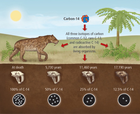
We can also use the concept of half-life to determine how long it will take for a given element to decay to some fraction of its original amount. This is the basis of radiometric dating. Carbon-14 is frequently used in radiocarbon dating, where by measuring the ratio of carbon-12 to carbon-14, scientists can reveal the age of ancient objects. Carbon-14 is created by high-energy cosmic rays interacting with Earth’s atmosphere. The carbon-14 is then absorbed by plants, thus entering the food chain. When living matter dies, it stops absorbing carbon, and the unstable carbon-14 decays, while the stable carbon-12 does not. If the amount of carbon-12 and carbon-14 were initially the same, then by finding the ratio today, we can find how old the object is.
(Ex 16.12, Pearson Physics) Consider carbon-14, which has a half-life of 5730 years. How long will it take for there to be 1/8 the original amount of carbon-14 remaining in a sample?
ANSWER
We know that the half-life of carbon-14 is 5730 years, and that from the decay equation: \(N = N_0\left(\frac{1}{2}\right)^{t/t_{1/2}} = \frac{1}{8}N_0\)
Thus for one-eighth to remain:
If we think in terms of half-lives, we can see that three half-lives will reduce the quantity by one-eighth, since
Thus,
It will take over 17 thousand years for \(7/8\) of carbon-14 to decay!
We could also solve this problem by looking at the decay curve of carbon-14.
%matplotlib inline

display('Here is the decay curve of carbon-14. We will use this graph to roughly determine how long it will take for 1/8 of the original amount to remain, or 12.5%.')

x=np.linspace(0,40000,1000)
plt.figure(figsize=(11,7));
plt.plot(x,N(100,x,5730), linewidth=2, color='#f4426e');
plt.title('Radioactive Decay Curve of Carbon-14', fontsize=20);
plt.xlabel('Time (years)', fontsize=18);
plt.ylabel('Carbon-14 Remaining (%)', fontsize=18);
plt.yticks(np.arange(0, 101, 10.0));
plt.xticks(fontsize=15);
plt.yticks(fontsize=15);
plt.xlim([0,40000]);
plt.ylim([0,100]);
plt.grid(alpha=0.8, linestyle = '--');
'Here is the decay curve of carbon-14. We will use this graph to roughly determine how long it will take for 1/8 of the original amount to remain, or 12.5%.'
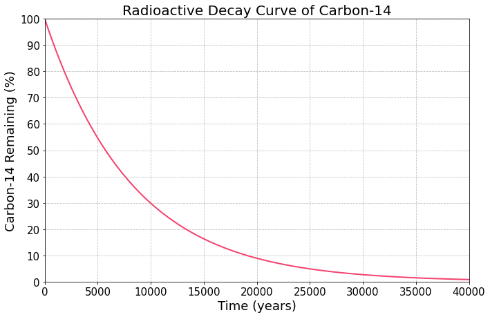
display("Let's pretend we don't know what the half-life of carbon-14 is. However, we do still know that after one half-life, 50% of our carbon-14 will remain. Let's mark this point on the graph.")

button_1 = widgets.Button(description='First half-life', disabled=False, tooltip='click me to continue', icon='')

def click_button_1(*args):
    button_1.disabled = True
    x=np.linspace(0,40000,1000)
    plt.figure(figsize=(11,7));
    plt.plot(x,N(100,x,5730), linewidth=2, color='#f4426e');
    plt.title('Radioactive Decay Curve of Carbon-14', fontsize=20);
    plt.xlabel('Time (years)', fontsize=18);
    plt.ylabel('Carbon-14 Remaining (%)', fontsize=18);
    plt.yticks(np.arange(0, 101, 10.0));
    plt.xticks(fontsize=15);
    plt.yticks(fontsize=15);
    plt.xlim([0,40000]);
    plt.ylim([0,100]);
    plt.grid(alpha=0.8, linestyle = '--');
    plt.plot(5730,50,'ko',markersize=6)
    plt.hlines(y=50, xmin=0.0, xmax=5730.0, color='k', linestyle = '--', linewidth=2)
    plt.vlines(ymin=0, ymax=50.0, x=5730, color='k', linestyle = '--', linewidth=2 )
    plt.text(300, 46,'one half-life')

button_1.on_click(click_button_1)
display(button_1)
"Let's pretend we don't know what the half-life of carbon-14 is. However, we do still know that after one half-life, 50% of our carbon-14 will remain. Let's mark this point on the graph."
display('After another half-life, another 50% of the remaining carbon-14 will decay. This means we will have 25% of the original amount we started out with.')

button_2 = widgets.Button(description='Second half-life', disabled=False, tooltip='click me to continue', icon='')

def click_button_2(*args):
    button_2.disabled = True
    plt.figure(figsize=(11,7));
    plt.plot(x,N(100,x,5730), linewidth=2, color='#f4426e');
    plt.title('Radioactive Decay Curve of Carbon-14', fontsize=20);
    plt.xlabel('Time (years)', fontsize=18);
    plt.ylabel('Carbon-14 Remaining (%)', fontsize=18);
    plt.yticks(np.arange(0, 101, 10.0));
    plt.xticks(fontsize=15);
    plt.yticks(fontsize=15);
    plt.xlim([0,40000]);
    plt.ylim([0,100]);
    plt.grid(alpha=0.8, linestyle = '--')
    plt.plot(5730,50,'ko',markersize=6)
    plt.hlines(y=50, xmin=0.0, xmax=5730.0, color='k', linestyle = '--', linewidth=2)
    plt.vlines(ymin=0, ymax=50.0, x=5730, color='k', linestyle = '--', linewidth=2 )
    plt.text(300, 46,'one half-life')
    plt.hlines(y=25, xmin=0.0, xmax=5730.0*2, color='b', linestyle = '--', linewidth=2)
    plt.vlines(ymin=0, ymax=25.0, x=5730*2, color='b', linestyle = '--', linewidth=2 )
    plt.text(5800, 17,'two half-lives', color='b')

button_2.on_click(click_button_2)
display(button_2)
'After another half-life, another 50% of the remaining carbon-14 will decay. This means we will have 25% of the original amount we started out with.'
display('After yet another half-life, another half of the remaining carbon-14 will decay. This means we will have 12.5% of the original amount we started out with - this is the quantity we are looking for!')
button_3 = widgets.Button(description='Third half-life', disabled=False, tooltip='click me to continue', icon='')
html_w=widgets.HTML()

def click_button_3(*args):
    button_3.disabled = True
    plt.figure(figsize=(11,7));
    plt.plot(x,N(100,x,5730), linewidth=2, color='#f4426e');
    plt.title('Radioactive Decay Curve of Carbon-14', fontsize=20);
    plt.xlabel('Time (years)', fontsize=18);
    plt.ylabel('Carbon-14 Remaining (%)', fontsize=18);
    plt.yticks(np.arange(0, 101, 10.0));
    plt.xticks(fontsize=15);
    plt.yticks(fontsize=15);
    plt.xlim([0,40000]);
    plt.ylim([0,100]);
    plt.grid(alpha=0.8, linestyle = '--')
    plt.plot(5730,50,'ko',markersize=6)
    plt.hlines(y=50, xmin=0.0, xmax=5730.0, color='k', linestyle = '--', linewidth=2)
    plt.vlines(ymin=0, ymax=50.0, x=5730, color='k', linestyle = '--', linewidth=2 )
    plt.text(300, 46,'one half-life')
    plt.hlines(y=25, xmin=0.0, xmax=5730.0*2, color='b', linestyle = '--', linewidth=2)
    plt.vlines(ymin=0, ymax=25.0, x=5730*2, color='b', linestyle = '--', linewidth=2 )
    plt.text(5800, 17,'two half-lives', color='b')
    plt.hlines(y=12.5, xmin=0.0, xmax=5730.0*3, color='m', linestyle = '--', linewidth=2)
    plt.vlines(ymin=0, ymax=12.50, x=5730*3, color='m', linestyle = '--', linewidth=2 )
    plt.text(10100, 5,'three half-lives', color='m')
    html_w.value="So, we have found that after 3 half-lives, 1/8 of the carbon-14 is remaining. Now we can read the date off the graph to find that three half-lives corresponds to approximately 17 000 years."

button_3.on_click(click_button_3)
display(button_3)
display(html_w)
'After yet another half-life, another half of the remaining carbon-14 will decay. This means we will have 12.5% of the original amount we started out with - this is the quantity we are looking for!'
Problems
Try the following problems on your own. You can always refer to the above examples if you get stuck!
1. Uranium-235 has a half-life of 703.8 million years. Suppose you find a large pile of rock containing 1kg of uranium-235 on a treasure hunt. Assume the pile formed at the same time the Earth did, approximately 4.6 billion years ago. How much uranium-235 was initially in the pile?
a1 = widgets.Text(placeholder = "Submit your answer here")
counter1 = 0

def callback(b):
    global counter1
    counter1 += 1
    if counter1 < 4:
        ans = b.value.replace(" ","").lower()
        if ans == "92.8kg":
            display(Latex("Great! The pile started out with 92.79 kg of uranium-235 when it was intially formed."))
            counter1 = 5
        else:
            display(Latex('Try again!'))
    elif counter1 == 4:
        display(Latex("The pile started out with 92.79 kg of uranium-235 when it was intially formed."))
        display(Latex('Here is the solution:'))
        display(Latex(r'$N = N_0\left(\frac{1}{2}\right)^{t/t_{1/2}}$, with $N = 1$ kg, $t = 4.6\times 10^{9}$ years, and $t_{1/2} = 703.8\times 10^6$ years. We are trying to find $N_0$, so we can simply rearrange the equation to find:'))
        display(Latex(r'$N_0 = \frac{N}{(1/2)^{4.6\times 10^9/703.8\times 10^6}}$'))
        display(Latex(r'$N_0 = 92.8$ kg'))


display(a1)
a1.on_submit(callback)
2. You are doing an experiment with radon-222. You initially have 6.2 grams of radon-222, and after 15.3 days, you have 0.3875 grams of radon-222 remaining. What is the half-life of radon-222, in seconds?
a2 = widgets.Text(placeholder = "Submit your answer here")
counter2 = 0

def callback(b):
    global counter2
    counter2 += 1
    if counter2 < 4:
        ans = b.value.replace(" ","").lower()
        if ans == '330480seconds':
            display(Latex(r"Great! Radon-222 has a half life of around $330 \times 10^3$ second, or 3.8 days."))
            counter2 = 5
        else:
            display(Latex('Try again!'))
    elif counter2 == 4:
        display(Latex(r"Radon-222 has a half life of around $330 \times 10^3$ second, or 3.8 days."))
        display(Latex('Here is the solution:'))
        display(Latex(r'We know what $N$, $N_0$, and $t$ are, so we need to solve for $t_{1/2}$ in the decay equation. To solve for the exponent, we would need use logarithms, which is beyond the scope of this notebook. Fortunately, in this case the amount of time that was passed is a multiplt of the half-life. We can determine this by taking the ratio of $N$ and $N_0$:'))
        display(Latex(r'$\frac{N}{N_0} = \frac{0.3875}{6.2} = 0.625$'))
        display(Latex(r'$0.625 = \frac{1}{16} = \frac{1}{2}\times\frac{1}{2}\times\frac{1}{2}\times\frac{1}{2} = \left(\frac{1}{2}\right)^4$'))
        display(Latex('Now, from the decay equation:'))
        display(Latex(r'$\frac{N}{N_0} = \left(\frac{1}{2}\right)^4 = \left(\frac{1}{2}\right)^{15.3/{t_{1/2}}}$'))
        display(Latex('So we know that'))
        display(Latex(r'$\frac{15.3}{t_{1/2}} = 4$'))
        display(Latex(r'$t_{1/2} = \frac{15.3}{4}$'))
        display(Latex(r'$t_{1/2} = 3.825$ days'))
        display(Latex('Now, all we have to do is convert our answer into seconds.'))
        display(Latex(r'$3.825$ days $\times 24$ hours/day $\times 60$ mins/hour $\times 60$ seconds/min = 330 480 seconds'))


display(a2)
a2.on_submit(callback)
3. On April 26, 1986 the Chernobyl Nuclear Power Plant suffered a catastrophic failure of one of its reactor cores. The disaster scattered deadly radioactive contamination around the globe. Some of the radioactive substances released were iodine-131, caesium-137, strontium-90, and plutonium-241, which in turn decays into americium-241. A 30 kilometer exclusion zone has been established surrounding the power plant to protect humans from absorbing any of the remaining deadly radiation.
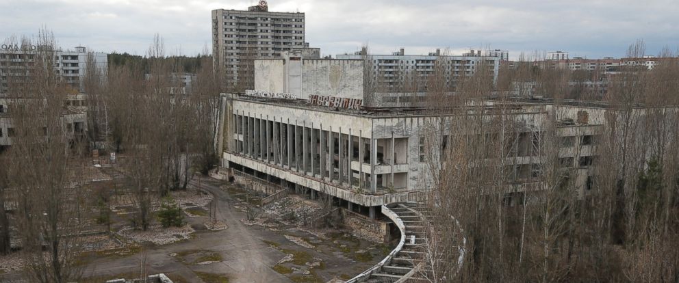
Assume that the exclusion zone will be safe to re-enter when the amount of radiation has reduced to \(7\times 10^{-13}\) % of its initial value immediately following the nuclear disaster. Look up the half-lives of the elements mentioned above here, and determine how long it will be before humans can safely re-enter this zone.
a3 = widgets.Text(placeholder = "Submit your answer here")
counter3 = 0

def callback(b):
    global counter3
    counter3 += 1
    ans = b.value.replace(" ","").lower()

    if ans == '20210years':
        display(Latex(r"Well done! 20,000 years is a rough estimate of how long until the radiation in the exclusion zone reached safe levels. "))
        counter3 = 5
    else:
        if counter3 == 1:
            display(Latex('Try again!'))
        if counter3 == 2:
            display(Latex(r'Try again! Hint: What element has the longest half-life? '))
        elif counter3 == 3:
            display(Latex(r'Try again! Hint: $\left(\frac{1}{2}\right)^{47} = 7\times10^{-13}$ %'))
        elif counter3 == 4:
            display(Latex(r"Recent estimates suggest in another 20,000 years the exlusion zone will be safe to re-enter. We can estimate this as follows:"))
            display(Latex('The longest-half life is of americium-241, at 430 years. As the hint mentioned, 47 half-lives of americium must pass for the radiation tp reach an acceptable level. Thus,'))
            display(Latex(r'$t = 47 \times t_{1/2}$'))
            display(Latex(r'$t = 47 \times 430$ years'))
            display(Latex(r'$t= 20210$ years'))


display(a3)
a3.on_submit(callback)
Graphing problems
For this problem, you will be presented with a table of data on the radioactivity of a sample material. You will need to graph the data to find
(a) the half-life of the material
(b) the initial amount at time t=0
In the next cell, we will work through some steps on how to create plots in python.
The following table shows the activity of a sample isotope at various times. Graph the following data to help you answer (a) and (b) above.
Time (years) |
Amount of isotope remaining (grams) |
|---|---|
25 |
3.04 |
50 |
2.32 |
75 |
1.76 |
100 |
1.32 |
125 |
1.00 |
150 |
0.76 |
175 |
0.58 |
200 |
0.44 |
display('To make a plot of the data, we need to first enter it in a form python can read. Input the time data with the following syntax:')
print('time = [25, 50, ...]')
display('Make sure that you enter the time entries in order from the top of the table to the bottom.')
time_check = 'time=[25,50,75,100,125,150,175,200]'
a = widgets.Text(placeholder = "Enter the time here")
counter4 = 0

def callback(b):
    global counter4
    ans = b.value.replace(" ","")
    if ans == time_check and counter4 < 5:
        time = [25, 50, 75, 100, 125, 150, 175, 200]
        display(Latex('Great! Now enter the "amount remaining" the same way, this time calling the variable amnt, i.e. "amnt = [...]"'))
        counter4 = 6
    elif counter4 < 6:
        counter4 += 1
        display(Latex('Try again!'))
        if counter4 == 1:
            display(Latex("Don't forget to type 'time = ' in the input box as well."))
        elif counter4 == 5:
            display(Latex("The correct input we were looking for was"))
            print('time = [25, 50, 75, 100, 125, 150, 175, 200]')
            time = [25, 50, 75, 100, 125, 150, 175, 200]

display(a)
a.on_submit(callback)
'To make a plot of the data, we need to first enter it in a form python can read. Input the time data with the following syntax:'
time = [25, 50, ...]
'Make sure that you enter the time entries in order from the top of the table to the bottom.'
You’ll use the box below in the next part of the question
display('Next, enter the amount of isotope remaining. Input the data with the following syntax:')
print('amnt = [3.04,2.32, ...]')
amnt_check = 'amnt=[3.04,2.32,1.76,1.32,1.00,0.76,0.58,0.44]'
b = widgets.Text(placeholder = "Enter the amount here")
counter5 = 0

def callback(j):
    global counter5
    ans = j.value.replace(" ","")
    if ans == amnt_check and counter5 < 5:
        display(Latex('Well done!'))
        amnt = [3.04, 2.32, 1.76, 1.32, 1.00, 0.76, 0.58, 0.44]
        counter5 = 6
    elif counter5 < 5:
        counter5 += 1
        display(Latex('Try again!'))
        if counter5 == 1:
            display(Latex("Don't forget to type 'amnt = ' in the input box as well."))
        elif counter5 == 5:
            display(Latex("The correct input we were looking for was"))
            print('amnt = [3.04, 2.32, 1.76, 1.32, 1.00, 0.76, 0.58, 0.44]')
            amnt = [3.04, 2.32, 1.76, 1.32, 1.00, 0.76, 0.58, 0.44]

display(b)
b.on_submit(callback)
'Next, enter the amount of isotope remaining. Input the data with the following syntax:'
amnt = [3.04,2.32, ...]
display('Now we can plot the data that you have enterd. We do this with the matplotlib library, which has already been imported into the notebook.')
display('To make a plot, we can call the "plot" function from the matplotlib library with the following command:')
print("plt.plot(time, amnt, linestyle='', marker = 'o', color = 'orange', markersize = 6)")
display("Try creating your own plot now with this command. Make sure you enter the correct variable for 'x' and 'y'! (i.e. 'time' and 'amnt')")
display("Feel free to try a different color or marker syle.")
P = widgets.Text(placeholder = "Define plot style here")
plot_rendered = False

def callback(b):
    global plot_rendered
    if plot_rendered:
        return
    plot_rendered = True
    time = [25, 50, 75, 100, 125, 150, 175, 200]
    amnt = [3.04, 2.32, 1.76, 1.32, 1.00, 0.76, 0.58, 0.44]
    plt.figure(figsize=(11,7))
    plt.grid(alpha = 0.8, linestyle = '--')
    plt.xticks(fontsize=15)
    plt.yticks(fontsize=15)
    plt.xlabel('Time (years)', fontsize=15)
    plt.ylabel('Amount Remaining (grams)', fontsize=15)
    plt.xlim([0,205])
    plt.ylim
    ans = b.value.replace(" ", "")
    if ans == "plt.plot(time,amnt,linestyle='',marker='o',color='orange',markersize=6)":
        display(Latex('Well done! You have successfully created a plot of the data in the above table. Use this plot to help answer the questions in the next cell!'))
        color_c='orange'
    else:
        display(Latex("Sorry, some of your plot arguments are't valid. We will apply the default parameters instead. For more information on what parameter are avaliable, visit: https://matplotlib.org/api/_as_gen/matplotlib.pyplot.plot.html"))
        color_c='blue'
    plt.plot(time, amnt, linestyle='',marker='o', color = color_c,markersize=6)

display(P)
P.on_submit(callback)
'Now we can plot the data that you have enterd. We do this with the matplotlib library, which has already been imported into the notebook.'
'To make a plot, we can call the "plot" function from the matplotlib library with the following command:'
plt.plot(time, amnt, linestyle='', marker = 'o', color = 'orange', markersize = 6)
"Try creating your own plot now with this command. Make sure you enter the correct variable for 'x' and 'y'! (i.e. 'time' and 'amnt')"
'Feel free to try a different color or marker syle.'
display('You will need to use the plot generated from the example in the cell above this one to answer the following questions. Make sure you go back and complete this question before moving on.')
display('(a) What is the half-life of the sample?')

h = widgets.Text(placeholder = "Submit your answer here")
counter6 = 0

def callback(b):
    global counter6
    ans = b.value.replace(" ","").lower()
    if ans == "63years" and counter6 < 5:
        display(Latex('Excellent!'))
        counter6 = 6
    elif counter6 < 5:
        counter6 += 1
        display(Latex('Try again!'))
        if counter6 == 5:
            display(Latex('The half-life of the sample is 63 years.'))

display(h)
h.on_submit(callback)
'You will need to use the plot generated from the example in the cell above this one to answer the following questions. Make sure you go back and complete this question before moving on.'
'(a) What is the half-life of the sample?'
display('(b) What was the initial quantity of the sample at t=0?')
a = widgets.Text(placeholder = "Submit your answer here")
counter7 = 0

def callback(b):
    global counter7
    ans = b.value.replace(" ","").lower()
    if ans == '4.0grams' and counter7 < 5:
        display(Latex('Perfect!'))
        counter7 = 6
    elif counter7 < 5:
        counter7 += 1
        display(Latex('Try again!'))
        if counter7 == 5:
            display(Latex('The sample intially had 4.0 grams of the element.'))

display(a)
a.on_submit(callback)
'(b) What was the initial quantity of the sample at t=0?'
Conclusion
The half-life of a radioactive substance is the time it takes for \(1/2\) of the substance to decay into it’s daughter element. How fast an element decays depends on how much of that element there is, resulting in an exponentially decaying relationship between the amount of an isotope remaining and how much time has passed.
It is possible to determine the half-life of an element based on a graph of its radioactive decay.
If the half-life of an element is known, it is possible to determine the age of the sample based upon what the initial amount of the element was. This forms the basis of radiometric and radiocarbon dating.
As a bonus, you should now also have some practice plotting data points in Python.
