Uniform Motion and Uniformly Accelerated Motion¶

Grade 11

https://giphy.com/gifs/usain-bolt-sgjJkkJutglMY

Introduction¶

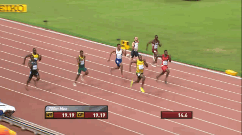
Everything in the universe is constantly moving. Objects can be moving incredibly slow, so slow that they appear to be at rest, or so incredibly fast that you may not even see it. Even if you’re standing still on Earth, you’re moving and incomprehensible speeds. On Earth, you are moving around the Sun at approximately 108,000 km/h, and the Sun is orbiting galactic center at approximately 720,000 km/h. But that’s not it: our galaxy the Milky Way is moving at approximately 2,268,000 km/h. As motion is so universal, understanding motion is an important topic of physics. Motion is defined by the change of position of an object with respect to other surrounding objects. For example a car is moving with respect to trees on the roadside. Motion can be described using three important quantities: velocity, speed and acceleration. In this notebook, we will familiarize ourselves with two types of motion: uniform motion, and uniformly accelerated motion.

Concepts of Uniform Motion¶

Motion is described by three variables: distance (\(d\)), velocity (\(\vec{v}\)), and acceleration (\(\vec{a}\)). Let’s define and explore these quantities below.

Distance Vs. Displacement¶

To begin, let us outline the difference between distance and displacement.

Distance describes the length of the actual path travelled to travel from one point to another.

Displacement is identical to distance as it describes the amount of space between two points. However, displacement is a vector quantity which means it also specifies the direction of travel, as well as the amount of space between two points.

Below is a video which demonstrates the difference between distance and displacement:

%%html
<iframe width="560" height="315" src="https://www.youtube.com/embed/u60JlEAGGWM" frameborder="0" allow="autoplay; encrypted-media" allowfullscreen></iframe>

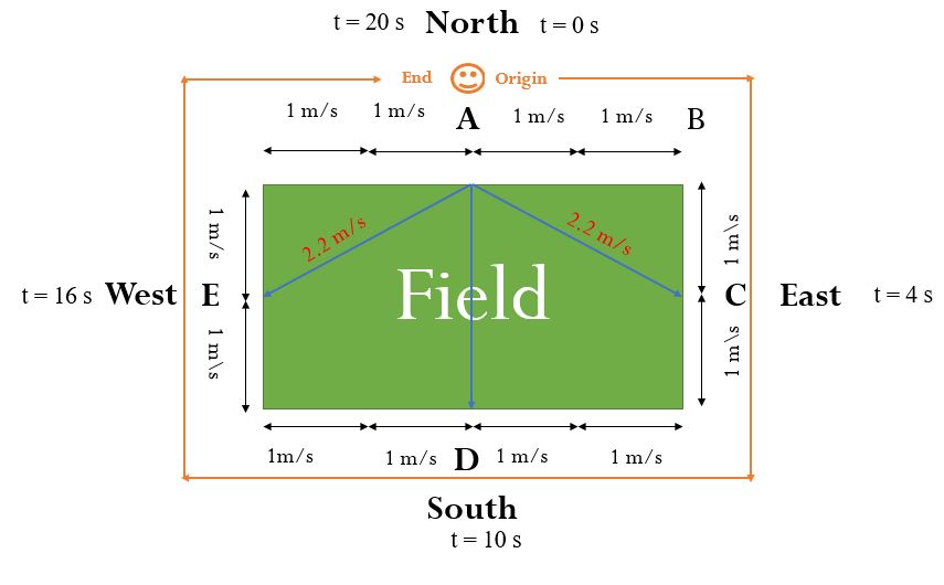
Practise

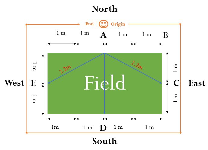
Calculate the distance and displacement based on the image below. Imagine you start at point \(\textrm{A}\) and you move around the field in the following order

\[\textrm{A} \rightarrow \textrm{B} \rightarrow \textrm{C} \rightarrow \textrm{D} \rightarrow \textrm{E} \rightarrow \textrm{A}\]

hide_me

def q_1(val):
    if val == "Distance: 2m and Displacement: 2m East":
        display(Latex("Correct!"))
        display(Latex("Displacement contains both measurement and direction"))
    elif val == ' ':
        None
    else:
        display(Latex("Try Again!"))

display("Calculate the distance and displacement at point B?")

a1 = 'Distance: 2m and Displacement: 2m'
a2 = "Distance: 2m and Displacement: 2m East"
a3 = "Distance: 2m North and Displacement: 2m"
interact(q_1, val = widgets.Dropdown(options=[' ',a1 ,a2, a3 ],value = ' ',description = 'Choose One:',disabled = False));

'Calculate the distance and displacement at point B?'

hide_me

def q_2(val):
    if val == "Distance: 9m North and Displacement: 2.2m NW":
        display(Latex("Correct!"))
        display(Latex("Distance: Actual path covered and Displacement: Shortest path covered with direction"))
    elif val == ' ':
        None
    else:
        display(Latex("Try Again!"))

display("Calculate the distance and displacement at point E?")

a1 = 'Distance: 9m and Displacement: 7m'
a2 = "Distance: 3m and Displacement: 2.2m NW"
a3 = "Distance: 9m North and Displacement: 2.2m NW"
interact(q_2, val = widgets.Dropdown(options=[' ',a1 ,a2, a3 ],value = ' ',description = 'Choose One:',disabled = False));

'Calculate the distance and displacement at point E?'

Speed Vs. Velocity¶

Analogous to distance and displacement are speed and velocity, however now these quantities also imply that the object’s distance/displacement is changing. Let’s take a look at how speed and velocity are defined.

Speed is the rate of change of distance over time.

\[ \begin{equation} \textrm{speed } = \frac{\textrm{change} \ \textrm{of} \ \textrm{distance (m)}}{\textrm{time (s)}} \end{equation} \]

Velocity is the rate of change of displacement over time.

\[\begin{split} \begin{equation} \textrm{velocity, } \vec{v} = \frac{\textrm{change} \textrm{ of} \textrm{ displacement (m)}}{\textrm{time (s)}} \\ \textrm{m} = \textrm{meter } \textrm{and} \textrm{ s} = \textrm{second} \end{equation} \end{split}\]

Practise

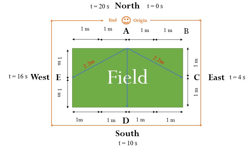
Now, let’s repeat a similar question as we did with displacement and distance, but now include velocity. The required time of one point to another point is given below:

\(\textrm{A} \rightarrow \textrm{C}: 4 \textrm{ sec}\)
\(\textrm{A} \rightarrow \textrm{D}: 10 \textrm{ sec}\)
\(\textrm{A} \rightarrow \textrm{E}: 16 \textrm{ sec}\)
\(\textrm{A} \rightarrow \textrm{A}: 20 \textrm{ sec}\)

hide_me

def q_1(val):
    if val == "Speed: 0.75 m/s and Velocity: 0.55 m/s NE":
        display(Latex("Correct!"))
        display(Latex("Velocity contains both measurement and direction as it relates to displacement"))
    elif val == ' ':
        None
    else:
        display(Latex("Try Again!"))

display("Calculate the speed and velocity at point C?")

a1 = 'Speed: 0.75 m/s and Velocity: 0.55 m/s NE'
a2 = "Speed: 0.55 m/s and Velocity: 0.75 m/s NE"
a3 = "Speed: 1 m/s and Velocity: 0.55 m/s NE"
interact(q_1, val = widgets.Dropdown(options=[' ',a1 ,a2, a3 ],value = ' ',description = 'Choose One:',disabled = False));

'Calculate the speed and velocity at point C?'

hide_me

def q_2(val):
    if val == "Speed: 0.60 m/s and Velocity: 0.20 m/s South":
        display(Latex("Correct!"))
        display(Latex("Speed and Velocity are not always equivalent"))
    elif val == ' ':
        None
    else:
        display(Latex("Try Again!"))

display("Calculate the speed and velocity at point D?")

a1 = 'Speed: 0.80 m/s and Velocity: 0.60 m/s South'
a2 = "Speed: 0.60 m/s and Velocity: 0.20 m/s South"
a3 = "Speed: 0.60 m/s and Velocity: 0.60 m/s South"
interact(q_2, val = widgets.Dropdown(options=[' ',a1 ,a2, a3 ],value = ' ',description = 'Choose One:',disabled = False));

'Calculate the speed and velocity at point D?'

Acceleration¶

Velocity can also change with respect to time. A change in velocity requires acceleration, which is defined as rate of change of velocity over time. As acceleration depends on the change in the vector quantity velocity, acceleration is also a vector. Below is an example of acceleration.

Acceleration is the rate of change of velocity over time. Acceleration is a vector quantity as it depends on velocity.

\[ \begin{equation} \textrm{acceleration, } \vec{a} = \frac{\textrm{change} \textrm{ of} \textrm{ velocity } (\frac{\text{m}}{\text{s}}) } {\textrm{time (s)}} \end{equation} \]

Here is an interactive animation demonstrating acceleration further.

Practice

Let’s go back to our field example and think about where we may see acceleration. Once again we are traveling from \(\textrm{A} \rightarrow \textrm{B} \rightarrow \textrm{C} \rightarrow \textrm{D} \rightarrow \textrm{E} \rightarrow \textrm{A}\):

hide_me

def q_1(val):
    if val == "Acceleration: 0 m/s\u00b2 East":
        display(Latex("Correct!"))
        display(Latex("No change in velocity and direction is also straight line"))
    elif val == ' ':
        None
    else:
        display(Latex("Try Again!"))

display("Calculate the acceleration at point B?")

a1 = 'Acceleration: 0 m/s\u00b2 East'
a2 = "Acceleration: 1 m/s\u00b2 East"
a3 = "Acceleration: 2 m/s\u00b2 East"
interact(q_1, val = widgets.Dropdown(options=[' ',a1 ,a2, a3 ],value = ' ',description = 'Choose One:',disabled = False));

'Calculate the acceleration at point B?'

hide_me

def q_1(val):
    if val == "Yes":
        display(Latex("Correct!"))
    elif val == ' ':
        None
    else:
        display(Latex("Try Again!"))

display("Does a change in direction imply that there was acceleration?")

a1 = 'Yes'
a2 = "No"

interact(q_1, val = widgets.Dropdown(options=[' ',a1 ,a2 ],value = ' ',description = 'Choose One:',disabled = False));

def q_2(val):
    if val == 'To change direction is to change your velocity, and this requires acceleration':
        display(Latex("Correct!"))
        display(Latex("Velocity is a vector quantity. To change your direction requires acceleration in another direction."))
    elif val == ' ':
        None
    else:
        display(Latex("Try Again!"))

display(Latex("Why?"))

a1 = 'To change direction is to change your velocity, and this requires acceleration'
a2 = 'When you change direction you gain speed, and this requires acceleration'


interact(q_2, val = widgets.Dropdown(options=[' ',a1 ,a2],value = ' ',description = 'Choose One:',disabled = False));

'Does a change in direction imply that there was acceleration?'

\[Why?\]

Uniform Motion¶

Now that we have an understanding of distance, displacement, velocity and acceleration, let’s use those quantities to describe “uniform motion”.

Uniform motion has the following two properties:

Motion is constant or steady that means object covers equal distance in equal time interval.
The object travels in a straight line.

Consider the blue car in the animation below

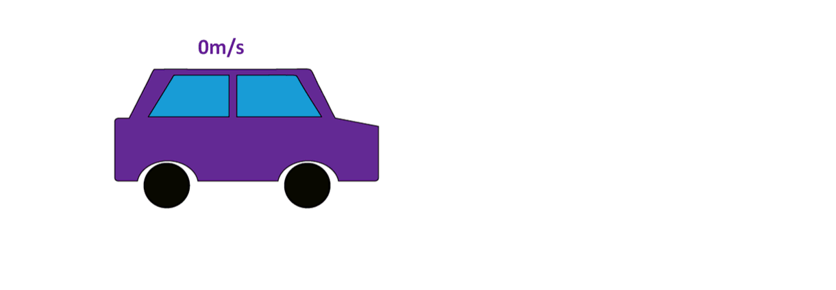
The blue car is travelling at a velocity of \(10 \textrm{ ms}^{-1}\) to the right. That means every second the car is travelling \(10 \textrm{ m}\). If we record this car’s displacement and velocity for \(10 \textrm{ sec}\), we get the following table.

Time \((sec\))	Displacement (\(m\))	Velocity (\(ms^{-1}\))
\( 1\)	\( 10\)	\(10\)
\( 2\)	\( 20\)	\(10\)
\( 3\)	\(30\)	\(10\)
\(4\)	\(40\)	\(10\)
\( 5\)	\( 50\)	\(10\)
\( 6\)	\( 60\)	\(10\)
\( 7\)	\(70\)	\(10\)
\(8\)	\(80\)	\(10\)
\( 9\)	\(90\)	\(10\)
\(10\)	\(100\)	\(10\)

We can also use this table to create the animation below:

hide_me

# Data
t = np.linspace(0,10,11)
d = np.linspace(0,100,11)
v = np.linspace(10,10,11)

# Create a figure with two subplots
fig, (ax1, ax2) = plt.subplots(1,2, figsize=(10, 4), dpi= 90, facecolor='w', edgecolor='k')

# Same X axis limt and grid initalizations
for ax in [ax1, ax2]:
    ax.set_xlim(0, 10)
    ax.grid()
    
ax1.set_ylim(0,100)
ax2.set_ylim(0,20)    

# Initialize the plot
l1, = ax1.plot([],[], 'go-', label='Displacement', linewidth=2)
leg = ax1.legend(loc='best')
l2, = ax2.plot([],[],  'rs-', label='Velocity')
leg = ax2.legend(loc='best')

fig.suptitle('Uniform Motion')
ax1.set_xlabel('Time (sec)')
ax2.set_xlabel('Time (sec)')
ax1.set_ylabel('Displacement (m)')
ax2.set_ylabel (r'$\mathrm{Velocity} \ (\mathrm{m/s})$')
             
# Initiate the animation
def animate(i):   
    l1.set_data(t[:i+1], d[:i+1])
    l2.set_data(t[:i+1], v[:i+1])
    
ani = FuncAnimation(fig, animate, interval = 800, frames=len(t))
plt.close()

# Convert animation to video
from IPython.display import HTML
HTML(ani.to_html5_video())

From the table and animations, we find that the blue car’s displacement is changing and its velocity is constant. This is an example of uniform motion. The car travels equal distance in equal time.

\[ \begin{equation} \textrm{velocity, } \vec{v} = \frac{\textrm{change} \ \textrm{of} \ \textrm{displacement (m)}}{\textrm{time (s)}} = \textrm{constant} \end{equation} \]

Based on your knowledge of uniform motion, what is the blue car’s acceleration?

hide_me

def q_1(val):
    if val == "0":
        display(Latex("Correct!"))
        display(Latex("Speed is constant and direction is in a straight line"))
    elif val == ' ':
        None
    else:
        display(Latex("Try Again!"))

a1 = '0'
a2 = 'Constant'
a3 = 'Variable'

interact(q_1, val = widgets.Dropdown(options=[' ',a1 ,a2, a3 ],value = ' ',description = 'Choose One:',disabled = False));

Uniform Accelerated Motion¶

hide_me

from IPython.display import HTML
# Youtube
#HTML('<iframe width="560" height="315" src="https://www.youtube.com/embed/JLm3JrCPtWs" frameborder="0" allow="autoplay; encrypted-media" allowfullscreen></iframe>')

%%html
<iframe width="560" height="315" src="https://www.youtube.com/embed/JLm3JrCPtWs" frameborder="0" allow="autoplay; encrypted-media" allowfullscreen></iframe>

Uniformly accelerated motion is a little different than the uniform motion we discussed earlier. In the case of uniformly accelerated motion, your velocity is increasing constantly and equally in time. Your velocity is changing in a way similar to how displacement changes if you’re traveling at constant velocity. Suppose you start at rest and begin running in order to catch a ball. In this scenario, you will need to accelerate. Suppose after each second, you are traveling 2 \(\frac{\textrm{m}}{\textrm{s}}\) faster than the second previous. In such a case, you have a uniform acceleration of 2 \(\frac{\textrm{m}}{\textrm{s}^2}\) (the seconds are squared in the units of acceleration as you are increasing your velocity constantly - i.e. you gain more velocity per second). Let’s write down displacement, velocity and acceleration as you try to catch this ball in a table:

Time \((\textrm{sec}\))	Displacement (\(\textrm{m}\))	Velocity (\(\textrm{ms}^{-1}\))	Acceleration (\(\textrm{ms}^{-2}\))
\( 0\)	\( 0\)	\(0\)	\(2\)
\( 1\)	\( 1\)	\(2\)	\(2\)
\( 2\)	\(4\)	\(4\)	\(2\)
\(3\)	\(9\)	\(6\)	\(2\)
\( 4\)	\(16\)	\(8\)	\(2\)
\(5\)	\(25\)	\(10\)	\(2\)
\(6\)	\(36\)	\(12\)	\(2\)
\( 7\)	\(49\)	\(14\)	\(2\)
\(8\)	\(64\)	\(16\)	\(2\)

Using the table, we can also create an animation

hide_me

# Data
t = np.linspace(0,8,9);
d = ([0,1,4,9,16,25,36,49,64]);
v = ([0,2,4,6,8,10,12,14,16]);
a = np.linspace(2,2,9);

# Create a figure with three subplots
fig, (ax1, ax2, ax3) = plt.subplots(1,3, figsize=(12.5, 4), dpi= 80, facecolor='w', edgecolor='k')

# Same X axis limt and grid initalizations
for ax in [ax1, ax2, ax3]:
    ax.set_xlim(0, 8);
    ax.grid();
    
ax1.set_ylim(0,70);
ax2.set_ylim(0,16);   
ax3.set_ylim(0,5);

# Initialize the plot
l, = ax1.plot([],[], 'go-', label='Displacement', linewidth=2);
leg = ax1.legend(loc='best');
l1, = ax2.plot([],[],  'rs-', label='Velocity');
leg = ax2.legend(loc='best');
l2, = ax3.plot([],[], 'b*-', label='Acceleration', linewidth=2);
leg = ax3.legend(loc='best');

fig.suptitle('Uniformly Accelerated Motion');
ax1.set_xlabel('Time (sec)');
ax2.set_xlabel('Time (sec)');
ax3.set_xlabel('Time (sec)');
ax1.set_ylabel('Displacement (m)');
ax2.set_ylabel (r'$\mathrm{Velocity} \ (\mathrm{m/s})$');
ax3.set_ylabel (r'$\mathrm{Acceleration} \ (\mathrm{m/s}^{2})$');

# Initiate the animation
def animate(i):
    l.set_data(t[:i+1], d[:i+1]);
    l1.set_data(t[:i+1], v[:i+1]);
    l2.set_data(t[:i+1], a[:i+1]);
    
ani=FuncAnimation(fig, animate, interval = 800, frames=len(t));
plt.close()

# Convert animation to video
from IPython.display import HTML
HTML(ani.to_html5_video())

Notice how with constant acceleration, your velocity increases linearly. As well, when you’re accelerating, your displacement changes parabolically. These relationships are explained further with the equations of motion below.

Equations of Motion¶

Using our relationships between displacement, velocity, acceleration and time, we can define “equations of motion” for a moving object. There are four such equations relevant to the principles of uniform motion and uniform acceleration.

Suppose an object with initial velocity \(\vec{\textrm{v}}_i\) \(\textrm{ms}^{-1}\) is travelling with uniform acceleration \(\vec{\textrm{a}}\) \(\textrm{ms}^{-2}\). After traveling a displacement \(\vec{\textrm{s}}\) in time \(\textrm{t}\) the object’s final velocity would be \(\vec{\textrm{v}_f}\) \(\textrm{ms}^{-1}\), these quantities are described by the following equations

\[ \begin{align} \vec{\textrm{v}_f}=\vec{\textrm{v}_i}+\vec{\textrm{a}} \textrm{t} \ \ \ \ \ \ \ \ (1) \ \ \ \ \ \ \ \ \ \ \ \ \ \ \ \ \ \ \ \ \ \ \ \ \ \vec{\textrm{s}} = (\frac{\vec{\textrm{v}_i}+\vec{\textrm{v}_f}}{2})\textrm{t} \; \; (2) \end{align} \]

\[ \begin{align} \vec{\textrm{s}} = \vec{\textrm{v}_i}\textrm{t}+\frac{1}{2}\vec{\textrm{a}}\textrm{t}^{2} \; (3) \ \ \ \ \ \ \ \ \ \ \ \ \ \ \ \ \ \ \ \ \ \vec{\textrm{v}_f} = \textrm{v}_i^{2}+2 \vec{\textrm{a}} \; \vec{\textrm{s}} \; \; \; \; (4) \end{align} \]

The equations above describe both uniform motion and uniformly accelerated motion. Equation (1) describes your final velocity given an intial velocity, and an acceleration over time. Notice how this is the equation of a line. This is what we see in the center plot of the animation above. Equation (3) describes your displacement moving at some initial velocity and accelerating uniformly for some time. Notice how time is squared in this equation. This means that this is the equation of a parabola. Equation (3) is what we see in the first plot of the animation above.

Mathematical Problems¶

As we work through the problems below, we will outline the following steps as we come to the solution. Breaking the problem down in this way makes the problem less intimidating, and makes the path to solution more straight foreward.

Identify and write what information is given in the problem, and the answer that we are asked for.

Using the information we know, and and the problem identified in step one, identify which equation(s) of motion we need to use to solve the problem.
Ensure that all the values are in the correct units and fill them in the selected equation.
Quote the answer and check the units.

Problem 1¶

A bus accelerates from rest at \(4 \textrm{ms}^{-2}\) until it reaches a final velocity of \(40 \ \textrm{ms}^{-1}\). For how many seconds was the bus accelerating?

Solution¶

Step 1:

Given,

initial velocity, \(\vec{\textrm{v}_i} = 0 \ \textrm{ms}^{-1}\)

final velocity, \(\vec{\textrm{v}_f} = 40 \ \textrm{ms}^{-1}\)

acceleration, \(\vec{\textrm{a}} = 4 \ \textrm{ms}^{-2}\)

time, \(\textrm{t} = ?\)

Step 2:

In this problem, the value of \(\vec{\textrm{v}_i}\), \(\vec{\textrm{v}_f}\) and \(\vec{\textrm{a}}\) are given and \(\textrm{t}\) is required. Now, check the above \(4\) motion equations, find the equation is related to\(\vec{\textrm{v}_i}\), \(\vec{\textrm{v}_f}\) and \(\vec{\textrm{a}}\) and \(\textrm{t}\). We find the equation and it is \(\vec{\textrm{v}_f} = \vec{\textrm{v}_i}+\vec{\textrm{a}}\textrm{t}\).

Step 3: After checking all the units of the given variable \(\textrm{v}_i\), \(\textrm{v}_f\) and \(\textrm{a}\), we find that they are correct. Then fill them in selected equation:

\[\begin{split} \begin{equation} \vec{\textrm{v}_f} = \vec{\textrm{v}_i}+\vec{\textrm{a}}\textrm{t} \\ \Rightarrow \vec{\textrm{a}}\textrm{t} = \vec{\textrm{v}_f} - \vec{\textrm{v}_i} \\ \Rightarrow \textrm{t} = \frac{\vec{\textrm{v}_f}-\vec{\textrm{v}_i}}{\vec{\textrm{a}}} \\ \Rightarrow \textrm{t} = \frac{40\textrm{ms}^{-1}-0\textrm{ms}^{-1}}{4\textrm{ms}^{-2}} \\ \Rightarrow \textrm{t} = 10\textrm{ s} \end{equation} \end{split}\]

Step 4:

time = \(10\textrm{ s}\) \((Ans)\)

This answer can be seen graphically in the animation below:

hide_me

# Data frame to create table
df = pd.DataFrame()
df['Velocity'] = np.arange(0,41,4)
df['Time'] = df['Velocity']/4

# Create a figure with two subplots
fig,(ax1,ax2) = plt.subplots(1,2,figsize=(6.8, 4), dpi= 100)

# Limit and label axis
ax1.set_ylim(0,10)
ax1.set_xlim(0,40)
ax1.set_xlabel('Velocity ($ms^{-1}$)')
ax1.set_ylabel('Time (s)')
ax1.grid()

# Initiate table properties
font_size=14
bbox=[0, 0, 1, 1]
ax2.axis('off')

# Initialize the plot
l, = ax1.plot([],[], 'go-', label='Time', linewidth=2)
leg = ax1.legend(loc='best')

# Initiate the animation
def animate(i):
    l.set_data(df['Velocity'][:i+1], df['Time'][:i+1])
    table = ax2.table(cellText = df.values[:i+1],bbox=bbox, colLabels=df.columns)
    
    
ani = FuncAnimation(fig, animate, interval = 800, frames=len(df.index))
plt.close()

# Convert animation to video
from IPython.display import HTML
HTML(ani.to_html5_video())

Problem 2¶

A car accelerates uniformly from \(16 \ \textrm{m/s}\) to \(38.8 \ \textrm{m/s}\) in \(3.1\) seconds. Calculate the distance travelled by the car.

Solution¶

Step 1:

Given,

\(\textrm{initial} \ \textrm{velocity}, \vec{\textrm{v}_i} = 16 \ \textrm{m/s}\)

\(\textrm{final} \ \textrm{velocity}, \vec{\textrm{v}_f} = 38.8 \ \textrm{m/s}\)

\(\textrm{time, t} = 3.1 \ \textrm{s}\)

\(\textrm{displacement, } \vec{\textrm{s}} = ?\)

Step 2:

Try yourself!

hide_me

display('Which equation can be chosen to solve this problem?')

#Create the box to select m=Motion of Equations
a=widgets.Checkbox(
    value=False,
    description=r"$\vec{\textrm{v}_f}=\vec{\textrm{v}_i}+\vec{\textrm{a}} \textrm{t}$",
    disabled=False
)

b=widgets.Checkbox(
    value=False,
    description=r'$\vec{\textrm{s}} = (\frac{\vec{\textrm{v}_i}+\vec{\textrm{v}_f}}{2})\textrm{t}$')

c=widgets.Checkbox(
    value=False,
    description=r'$\vec{\textrm{s}} = \vec{\textrm{v}_i}\textrm{t}+\frac{1}{2}\vec{\textrm{a}}\textrm{t}^{2}$'
)
d=widgets.Checkbox(
    value=False,
    description=r'$\vec{\textrm{v}_f} = \vec{\textrm{v}_i}^{2}+2 \vec{\textrm{a}} \; \vec{\textrm{s}}$',
    disabled=False
)

#Display the check box
display(a)
display(b)
display(c)
display(d)

#create a button to check the answer
button_check = widgets.Button(description="check")
display(button_check)

#Check the answer
def check_button(x):
    if a.value==False and b.value==True and c.value==False and d.value==False:
        display(Latex("Correct. Well done!"))
    else: 
        display(Latex("Wrong one!"))

button_check.on_click(check_button)

'Which equation can be chosen to solve this problem?'

hide_me

def q_1(val):
    if val == "84.94 m":
        display(Latex("Correct!"))
        display(Latex(r'$\vec{\textrm{s}} = (\frac{\vec{\textrm{v}_i}+\vec{\textrm{v}_f}}{2})\textrm{t}$'))
        display(Latex(r'$\vec{\textrm{s}} = (\frac{(16 + 38.8)} {2} \times 3.1) \textrm{ m}$'))
        display(Latex(r'$\vec{\textrm{s}} = 84.94 \textrm{ m}$'))
    elif val == ' ':
        None
    else:
        display(Latex("Try Again!"))

display("What is your final displacement?")

a1 = '84.94 m'
a2 = '65.26 m'
a3 = '89.5 m'

interact(q_1, val = widgets.Dropdown(options=[' ',a1 ,a2, a3 ],value = ' ',description = 'Choose One:',disabled = False));

'What is your final displacement?'

Problem 3¶

A racing car is traveling with a velocity of \(72 \ \textrm{km/h}\) N and accelerates at \(5 \ \textrm{m/s}^{2}\) for \(10 \ \textrm{s}\) N. What is the final velocity of the car and how far will it travel as it accelerates?

Solution¶

Step 1:

Given \(\textrm{initial} \ \textrm{velocity,} \vec{\textrm{v}_i} = 72 \ \textrm{km/h}\) N

\(\textrm{acceleration, } \vec{\textrm{a}} = 5 \ \textrm{m/s}^{2}\) N

\(\textrm{time}, \textrm{t} = 10 \ \textrm{s}\)

\(\textrm{final} \ \textrm{velocity}, \vec{\textrm{v}_f} = ?\)

\(\textrm{displacement}, \vec{\textrm{s}} = ?\)

Step 2: Let’s try,

hide_me

display('Which equations can be chosen to solve this problem?')

#Create the box to select m=Motion of Equations
a=widgets.Checkbox(
    value=False,
    description=r"$\vec{\textrm{v}_f}=\vec{\textrm{v}_i}+\vec{\textrm{a}} \textrm{t}$",
    disabled=False
)

b=widgets.Checkbox(
    value=False,
    description=r'$\vec{\textrm{s}} = (\frac{\vec{\textrm{v}_i}+\vec{\textrm{v}_f}}{2})\textrm{t}$')

c=widgets.Checkbox(
    value=False,
    description=r'$\vec{\textrm{s}} = \vec{\textrm{v}_i}\textrm{t}+\frac{1}{2}\vec{\textrm{a}}\textrm{t}^{2}$'
)
d=widgets.Checkbox(
    value=False,
    description=r'$\vec{\textrm{v}_f} = \vec{\textrm{v}_i}^{2}+2 \vec{\textrm{a}} \; \vec{\textrm{s}}$',
    disabled=False
)

#Display the check box
display(a)
display(b)
display(c)
display(d)

#create a button to check the answer
button_check = widgets.Button(description="check")
display(button_check)

#Check the answer
def check_button(x):
    if a.value==True and b.value==True and c.value==True and d.value==True:
        display(Latex("Correct. Well done!"))
        display(Latex("yes, all the equations can be used. It depends on which one you are picking.")) 
    else: 
        display(Latex("Try Again!"))
        display(Latex('Hint: More than one answers'))      

button_check.on_click(check_button)

'Which equations can be chosen to solve this problem?'

Step 3:

\[ \begin{equation} \textrm{initial} \ \textrm{velocity,} \vec{\textrm{v}_i} = 72 \ \textrm{km/h} N = \frac{72\times1000}{3600} \ \textrm{m/s} = 20 \ \textrm{m/s} \; N \end{equation} \]

Calculate final velocity,

\[\begin{split} \begin{equation} \vec{\textrm{v}_f} = \vec{\textrm{v}_i}+\vec{\textrm{a}}\textrm{t} \\ \vec{\textrm{v}_f}= 20+(5\times10) \\ \vec{\textrm{v}_f}= 70 \ \textrm{m/s} N \end{equation} \end{split}\]

Calculate displacement,

\[\begin{split} \begin{equation} \vec{\textrm{s}} = \vec{\textrm{v}_i}\textrm{t}+\frac{1}{2}{\vec{\textrm{a}}}{\textrm{t}^{2}} \\ \vec{\textrm{s}}=20\times10+\frac{1}{2}{5\times}{10^{2}} \\ \vec{\textrm{s}}=(200+250)\ \textrm{m} \\ \vec{\textrm{s}}=450 \ \textrm{m} \; N \end{equation} \end{split}\]

Step 4:

\[\begin{split} \begin{align} \textrm{final} \ \textrm{velocity}, \vec{\textrm{v}_f}=70 \ \textrm{m/s}\ \; N \;\;(Ans) \\ \textrm{displacement} = 84.94 \ \textrm{m} \ \; N \;\; (Ans) \end{align} \end{split}\]

Problem 4¶

An Air Canada plane requires a takeoff speed of \(78.5 \ \textrm{m/s}\) and \(1690 \ \textrm{m}\) of runway to reach that speed. Determine the acceleration of this plane and the time required to reach this speed.

Solution¶

Step 1: Let’s try,

hide_me

display('Which values are given in this problem?')

#Create the box to select m=Motion of Equations
a=widgets.Checkbox(
    value=False,
    description=r"$\vec{\textrm{v}_i}$",
    disabled=False
)

b=widgets.Checkbox(
    value=False,
    description=r'$\vec{\textrm{v}_f}$')

c=widgets.Checkbox(
    value=False,
    description=r'$\vec{\textrm{a}}$'
)
d=widgets.Checkbox(
    value=False,
    description=r'$\vec{\textrm{s}}$',
    disabled=False
)

e=widgets.Checkbox(
    value=False,
    description=r'$t$',
    disabled=False
)


#Display the check box
display(a)
display(b)
display(c)
display(d)
display(e)

#create a button to check the answer
button_check = widgets.Button(description="check")
display(button_check)

#Check the answer
def check_button(x):
    if a.value==True and b.value==True and c.value==False and d.value==True and e.value==False:
        display(Latex("Correct. Well done!"))
        display(Latex("Initial velocity is also given as initially plane will start from $0$ $ms^{-1}$"))
    else: 
        display(Latex("Wrong one!"))
          

button_check.on_click(check_button)

'Which values are given in this problem?'

Step 2:

\[ \begin{align} \textrm{Motion} \ \textrm{equation, } \vec{\textrm{v}_f} = \vec{\textrm{v}_i}^{2}+2 \vec{\textrm{a}} \; \vec{\textrm{s}} \textrm{ and } \vec{\textrm{v}_f}=\vec{\textrm{v}_i}+\vec{\textrm{a}} \textrm{t} \end{align} \]

Step 3

Let’s calculate,

hide_me

def q_1(val):
    if val == "acceleration = 1.82 ms\u00b2 and time = 43.06 s":
        display(Latex("Correct!"))
    elif val == ' ':
        None
    else:
        display(Latex("Try Again!"))

display("What is the plane's required acceleration, and how long was it accelerating?")

a1 = 'acceleration = 1.91 ms\u00b2 and time = 48.1 s'
a2 = 'acceleration = 1.82 ms\u00b2 and time = 43.06 s'
a3 = 'acceleration = 1.82 ms\u00b2 and time = 45.4 s'

interact(q_1, val = widgets.Dropdown(options=[' ',a1 ,a2, a3 ],value = ' ',description = 'Choose One:',disabled = False));

"What is the plane's required acceleration, and how long was it accelerating?"

Exercise¶

Question 1: A car starting from rest in straight moves with uniform acceleration of \(5 \ \textrm{ms}^{-2}\). What will be the velocity while crossing a person at a distance \(40 \ \textrm{m}\)? (Ans: \(20 \ \textrm{ms}^{-1}\))

Question 2: A bike accelerates uniformly from rest to a speed of \(1 \ \frac{\textrm{km}}{\textrm{min}}\) over a distance of \(65 \ \textrm{m}\). Determine the acceleration of the bike. (Ans: \(2.137 \ \textrm{ms}^{-1}\))

Question 3: A bullet leaves a rifle with a velocity of \(521 \ \textrm{ms}^{-1}\). While accelerating through the barrel of the rifle, the bullet moves a distance of \(0.840 \ \textrm{m}\). Determine the acceleration of the bullet (Consider a uniform acceleration). (Ans: \(1.62 \times 10^{5} \ \textrm{ms}^{-1}\))

Question 4: The Velocity of a jeep decreases uniformly from \(35 \ \textrm{ms}^{-1}\) and after \(8 \ \textrm{s}\) it becomes \(10 \ \textrm{ms}^{-1}\). Find the acceleration of the car? (Ans: \(-3.125 \ \textrm{ms}^{-2}\), You do not have worry about the ‘-‘ sign. It defines the direction as velocity is decreasing)

Conclusion¶

In this notebook, we introduced two important concepts of motion: Uniform and Uniformly accelerated motion. We demonstrated how motion is related to distance, speed, velocity and acceleration. We also showed the various linear relationships between displacement, velocity and uniform acceleration using both the equations of motion, and the graphs of those functions. Using these equations, we then demonstrated several cases where they we can apply the ideas of uniform motion and uniformly accelerated motion to solve classic physics problems. This notebook serves as an introduction to the concept of uniform and uniformly accelerated motion, and will allow you to solve a great many problems using these concepts, and should act as a reasonable primer for more complex kinematic problems.

Callysto Curriculum Notebooks

Uniform Motion and Uniformly Accelerated Motion¶

Introduction¶

Concepts of Uniform Motion¶

Distance Vs. Displacement¶

Speed Vs. Velocity¶

Acceleration¶

Uniform Motion¶

Uniform Accelerated Motion¶

Equations of Motion¶

Mathematical Problems¶

Problem 1¶

Solution¶

Problem 2¶

Solution¶

Problem 3¶

Solution¶

Problem 4¶

Solution¶

Exercise¶

Conclusion¶