

![]()
Nuclear Decay - Half Life
The half-life of an unstable atom is the amount of time required on average for half of a population of that atom to decay to a different element. The half-life can range from yottoseconds (\(10^{24}\) seconds!) to numbers so large that it’s hard to consider the atom unstable (for example Tellerium-128 has a half-life of approximately \(10^{24}\) (yotta) years). A short list of select atomic half-lives is available from Wikipedia here.
As an example, suppose you have a collection of one thousand atoms which have a half-life of twenty minutes. After twenty minutes your collection of those atoms will have shrunk to approximately five hundred atoms. However, that does not mean that your atoms have disappeared. Those unstable atoms have decayed, meaning that the atom has lost energy by emitting radiation and changed either its number of neutrons, protons, or both! Most commonly atoms decay by emitting a electrons, neutrons, positrons, or alpha particles (which are helium nuclei, He\(^{2+}\)). What happens in each of these decay processes is outlined below.
Modes of decay
Alpha (\(\alpha\)) Decay
Alpha decay is a decay process in which an atom releases an \(\alpha\) particle. An \(\alpha\) particle is simply another name for an ionized (no electrons) helium atom \(\left(^4_2He\right)\), so if an element undergoes alpha decay, the atom reduces its number of neutrons \(N\), and the number of protons \(Z\). In general, for an atom X with atomic number \(A\), the sum of neutrons and protons, decaying into an atom \(Y\) via \(\alpha\) decay has the following form:
Here \(A\) is the atomic number of an atom, or the sum of its number of neutrons \(N\) and protons \(Z\).
Alpha decay, written in terms of a concrete example, the \(\alpha\) decay of Uranium-235 would appear as
Where we see that uranium-235 decays to Thorium-231 by emitting an \(\alpha\) particle, it alpha decays. Notice however, that the total number of neutrons and protons are equal on both the right hand side and the left hand side of the reaction. Generally speaking however, the number of neutrons is not typically written explicitly, and calculated by subtracting \(Z\) from \(A\).
Beta \(\beta\) Decay
\(\beta\) decay comes in two flavors: beta positive (\(\beta^+\)) decay and beta minus (\(\beta^-\)) decay. \(\beta^-\) decay emits an electron, and \(\beta^+\) decay emits the anti-particle of the electron: the positron (a particle with the same mass, but opposite charge of an electron). In the case of \(\beta^+\) decay, the element emits a positron from a proton, therefore the atom ‘loses’ a proton and ‘gains’ a neutron. In the case of \(\beta^-\) decay, a neutron emits an electron meaning the atom ‘loses’ a neutron and ‘gains’ a proton.
They also emit mysterious and common particle known as a neutrino
The Neutrino
Beta Minus decay
Generally speaking \(\beta^-\) decay has the following form
where \(\bar{\nu}\) is an anti-neutrino. Notice that charge and mass is conserved. From the above formula, we see that a neutron is emitting an electron and anti-neutrino and then becomes a proton. Notice how both charge and mass is conserved, we gained a positive charge with the proton, but also gained a negative charge in the process with an electron.
Beta plus decay
where \(\nu\) is a neutrino. Notice that charge and mass is again conserved. From the above formula, we see that a proton is emitting a positron and neutrino, and the becomes a neutron.
Electron Capture
This wasn’t in the Alberta curriculum thing but would it important? There’s also a whole bunch of others that we could toss in here that could be considered optional. I kind of want to put it in because then the neutron capture stuff will make more sense. Not that that’s required either, but it would make for a cool animation.
Some Mathematical Background
Let’s build on our earlier discussion and start introducing some mathematical rigor to our discussion of half life. The half-life of an atom is denoted as \(\tau_{1/2}\), measured in seconds, where \(\tau\) is the Greek letter tau. Using the half life of an atom, we can calculate the number of atoms as a function of time \(N(t)\) with the following relationship
Where \(N(t)\) is the number of atoms you have at time \(t\), \(N_0\) is the original number of atoms at \(t=0\) and \(\lambda\) is known as the “half life constant” which has units of inverse seconds. The half life constant is a bit of an abstraction from the more intuitive half life, however \(\lambda\) is related to the half life by the following simple relationship
The above two equations make it is possible to calculate the amount of atoms remaining at any given time, provided the half life and the original number of atoms is known. Another, more subtle, fact about equation \ref{eq:decay} that is worth pointing out is that the exponential part (\(2.718^{\lambda t}\)) of that equation is directly related to the probability that an atom will decay at a given time. Intuitively this makes sense, which we illustrate with an example. Suppose we started with one thousand atoms, and after ten seconds we find that we only have 60% of our atoms remaining. Using equation \ref{eq:decay} we can write this scenario as follows with \(N_0 = 1000\)
We can manipulate the left hand side of this equation to show
Where if we substitute our new expression for \(N(t = 3 \text{ s})\) back to equation \ref{eq:probrelat}, we see that this function is analogous to a probability. In other words, the expression
is the probability that an atom will not decay at a given time \(t\), or
Where \(P_{exists}(t)\) is the probability that an atom will exist at time \(t\).
Now that we have an expression for the probability that an atom will not decay, we can now calculate the probability that an atom does decay. The probability that an atom does decay is simply one minus the probability of it not decaying, or
Where \(P_{decayed}(t)\) is the probability that an atom has decayed by time \(t\).
This means that the expression in equation \ref{eq:decay} is a “smooth idealization”. Radioactive decay is a statistical process, and actual data will only ever approach the solution of equation \ref{eq:decay}. In reality, our observations of radioactive will randomly fluctuate around that solution. To visualize this, we can use Python to get an idea of what we may measure if we were to observe an actual population of atoms decay.
Python Example
Using the relationships defined in equations \ref{eq:exist} and \ref{eq:decayed}, it is possible to construct a simple model to visualize how a population of atoms may be observed to decay. This is the case because we know the probability that an atom will decay or not at any given time step. If we know the probability of decay, we simply need to compare this probability to some metric in order to decide if our atom decays or not.
Sounds simple, but that’s not an obvious metric to know. How do you decide which atoms decay? Suppose we have an atom that has a 40% probability of decay, how exactly do we decide if this atom decays at a given time or not? Do we simply consider a large group of these atoms and choose 40% of them and say they have decayed? This is certainly an option, however, if we do it this way we won’t be observing the interesting random statistical fluctuations, as we would simply be using definition of equation \ref{eq:decay}. What methodology should we use in order to view actual fluctuations?
Radioactive decay as an analogy to tossing a biased coin
Suppose you were sifting through a bag of atoms and deciding which ones decay by throwing them away according to their half life. Let’s suppose that at your current instance in time, each atom has a 50% probability of decay. Doing this manually, conceivably you could pick an atom and flip a coin to decide its fate. If the coin showed heads you could keep the atom (the atom does not decay), and if the coin showed tails you could throw it away (the atom decays). Once you’ve gone through the entire set of atoms, you will have thrown away those atoms randomly according to their probability of decay. This is a reasonable methodology: you’re still removing half of the atoms randomly, and the act of removing one atom is completely independent from the act of removing another. Is there some way to generalize this process and apply it to what we’ve learned about nuclear decay?
Luckily, Python allows us to draw random numbers which are uniformly distributed between 0 and 1 algorithmically. In other words, there is a Python function which allows us to randomly draw a percentage between 0 and 100%, where each percentage is equally probable to draw. Using this function, we can compare our new random percentage, against our probabilities of decay to decide if our atom decays or not! This is exactly the same as flipping a coin for each atom, except now we’re using a “biased coin” which can favor heads over tails (or in our case decaying or not decaying). That’s still pretty abstract in terms of what this actually means. For an introduction to simulating a biased coin toss please see coin flipping for a brief introduction. Of course, if a deeper understanding of how the simulation of nuclear decay is not of interest to you, the following section is not required and you can feel free to skip the next section.
Simulating nuclear decay
The way in which we look through our “bag” of atoms can be depicted as a flow chart as seen below
Here we see the flowchart for the process of simulating nuclear decay. Here we see that for every instance in time \(t_i\) we have some number of atoms \(N\). At that instance in time, we compare the probability of decay for each atom to a unique random number \(r\). If the random number is less than our probability of decay, then the atom is said to have decayed. We then remove that atom from the bag. Once we have checked every atom at a particular instance in time, we now move to our next instance in time with our new number of atoms \(N\) and repeat the process
The pseudo-code below shows how you would write this process with in code. Here we’re looking through our “bag” of atoms, then the comparison between the random number and our calculated probability of decay acts as a (biased) coin toss to decide if the atom decays or not.
for each instance_in_time in time:
    probability_of_decay = 1 - exp(-lambda * instance_in_time)
    for each atom in atoms:
        # This is a random number between 0 and 1
        random_percent = random_number()
        if prob_decay > r:
            atom.decays()
Where here instance_in_time is an equally spaced time step (steps of one second for example), and we’re looping over many time steps. At each time step, we then calculate the probability that an atom decays at that instance in time by equation 5. We then loop over all atoms, generate a random number between 0 and 1 (random percentage between 0 and 100) and use that to decide if an atom decays on an atom to atom basis. Then, we do it again at the next time step. In terms of the coin toss analogy if probability_of_decay is greater than random_percent, our coin is heads and the atom does not decay. Should probability_of_decay be less than random_percent then our coin toss is tails and the atom decays.
To illustrate this with an example, if probability_of_decay is 76%, and the random number random_percent was 45%, our atom would not decay, however, if random_percent was greater than 76%, the atom would decay. As the random numbers are uniformly distributed, that means that each percentage between 0 and 100 are all equally probable.
An important thing to notice that we calculate the probability of decay before we enter the loop where we see if an atom decays or not. This is because at a single instant of time, the probability of decay for each atom is independent: if one atom decays, this does not affect if any of the others also decay.
What to keep in mind here is that the basis behind this simulation is deceptively simple: We’re simply deciding if each atom decays by flipping a biased coin at each step in time. If you were to do this “by hand” you would quite literally just be flipping coins and counting atoms. And that’s precisely what our simulation is doing, just faster than we can.
Below, we see an example of this simulation behavior for carbon-15, which has a half-life of 2.249 seconds.
For each step in time, we need to check if each atom decays or not. We only calculate our probability once because at a single instant in time, the probability of decay is the same for each – they are independent events.
import matplotlib.pyplot as plt
%matplotlib inline
import numpy as np
import random
import pandas as pd

def HalfLifeEquation(N_0, lamb, t):
    return N_0 * 2.71828 ** (-lamb * t)

t = np.linspace(0,4*2.449,500) # Halflife of carbon-15 is 2.249 seconds
plt.figure(figsize=(3, 2), dpi= 175, facecolor='w', edgecolor='k')
plt.plot(t, HalfLifeEquation(1000, np.log(2)/2.249, t), label="Predicted")
plt.ylabel("Number of atoms")
plt.xlabel("t (seconds)")
plt.title("Carbon 15 Decay")

def Decay(N_0, lamb,max_time, steps=100):
    time_atom_pairs = []
    N = N_0
    time_step = max_time/steps
    t = 0
    for i in range(steps):
        # the equation from eariler, divide by N to reuse function
        p = 1 - HalfLifeEquation(N, lamb, time_step)/N
        for i in range(N):
            # a 'random' number between 0 and 1 to compare to our decay probability
            r = random.uniform(0,1)
            if r < p: # if our decay probability for the atom is greater, that atom decays.
                N = N -1
            if N == 0: # if we run out of atoms we should stop
                break
        # We have now moved forward in time once again!
        t = t + time_step
        # Store how many atoms at a given time t we have in an array.
        time_atom_pairs.append([N, t])
    return time_atom_pairs
decays = Decay(1000, np.log(2)/2.249, 10, steps=500)

y,x = np.array(decays).T
plt.plot(x, y, label = "Simulated")
plt.legend()
plt.show()
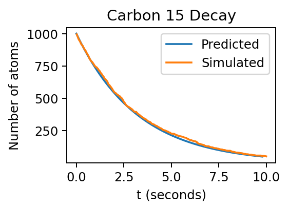
From the plot above we see that the simulated curve (orange) follows the predicted one (blue), but does not follow it exactly. This is a result of atomic decay being a statistical process.
Simulations
Below you have a widget where you can compare how quickly different atoms decay, and view a simulation of how that process would look if you were to observe these counts yourself. The data is pulled automatically from the National Institutes of Standards.
You can choose which isotopes to watch their decay with the element drop-down menus, and you can run for more or less time with the Time_Scale slider. Move the slider around at the bottom to advance the decay simulation forward or backwards in time.
Using the data
url = 'https://www.nist.gov/pml/radionuclide-half-life-measurements/radionuclide-half-life-measurements-data'
df = pd.read_html(url)[0]

# Rename the columns
df.columns = ["Radionuclide",
              "NumberOfSources",
              "HalfLifes_Followed",
              "HalfLife",
              "StandardUncertainty",
              "OtherUncertainty",
              "ref"]
df = df.drop(['ref', 'OtherUncertainty'], axis=1)
df
| Radionuclide | NumberOfSources | HalfLifes_Followed | HalfLife | StandardUncertainty | |
|---|---|---|---|---|---|
| 0 | 3H | 18 | 3 | 4500 ± 8 d | 8.00000 |
| 1 | 18F | 3 | 13.1 | 1.82951 ± 0.00034 h | 0.00024 |
| 2 | 22Na | 5 | 1.9 - 4.7 | 950.97 ± 0.15 d | 0.09000 |
| 3 | 24Na | 14 | 1.1 - 7.6 | 14.9512 ± 0.0032 h | 0.00090 |
| 4 | 32P | 2 | 2.8 | 14.263 ± 0.003 d | 0.00300 |
| ... | ... | ... | ... | ... | ... |
| 60 | 202Tl | 1 | 1.4 | 12.466 ± 0.081 d | 0.08100 |
| 61 | 203Hg | 14 | 1.7 - 6.6 | 46.619 ± 0.027 d | 0.00700 |
| 62 | 203Pb | 7 | 1.8 - 2.8 | 51.923 ± 0.037 h | 0.01300 |
| 63 | 207Bi | 2 | 0.9 | 11523. ± 15. d | 9.00000 |
| 64 | 228Th | 6 | 1.7 - 8.3 | 698.60 ± 0.36 d | 0.14000 |
65 rows × 5 columns
Once the data is tabulated, we can use it in combination with equation 1 we can create the theoretical traces, and use it in combination with equation 5 to generate our “observed” decay path. These are shown graphically with the widget below
Feel free to simulate decay over a longer time frame by adjusting Time_Scale and changing the decay isotope using the drop down menus.
from ipywidgets import interactive
import plotly as py
import plotly.graph_objs as go
py.offline.init_notebook_mode()

# Read and calculate the half-life of each element in the data frame.
def get_halflife(Element):
    multiplies = {'s':1., "min":60., "h":3600., "d":3600.*24.}
    index = index1 = np.where(df["Radionuclide"] == Element)[0][0]
    data = df["HalfLife"].iloc[index]
    half_life, pm, d_time, unit = data.split()
    scale = multiplies[unit]
    HalfLife = float(scale) * float(half_life)
    return HalfLife, unit

# calculate and animate the decay of two atoms on the same graph
def DecayRace2(Element1, Element2, Time_Scale=1):
    N_0 = 1000
    Decay_Points = 75
    # Grab the half-lives
    HalfLife_Element_1, unit1 = get_halflife(Element1)
    HalfLife_Element_2, unit2 = get_halflife(Element2)
    time_length = max(HalfLife_Element_1, HalfLife_Element_2)
    # Points for antimation of decay
    Points_Element_1 = Decay(N_0, np.log(2)/(float(HalfLife_Element_1)),
                      max_time= Time_Scale * float(time_length), steps=Decay_Points)
    Points_Element_2 = Decay(N_0, np.log(2)/(float(HalfLife_Element_2)),
                      max_time= Time_Scale * float(time_length), steps=Decay_Points)
    # Make Points
    y1,x1 = np.array(Points_Element_1).T
    y2,x2 = np.array(Points_Element_2).T
    # For the predicted traces
    t = np.linspace(0, Time_Scale * float(time_length), Decay_Points)
    y3 = HalfLifeEquation(N_0, np.log(2)/(float(HalfLife_Element_1)), t)
    y4 = HalfLifeEquation(N_0, np.log(2)/(float(HalfLife_Element_2)), t)
    Decay_Element_1 = go.Scatter(x = x1, y = y1, mode="markers+lines")
    Decay_Element_2 = go.Scatter(x = x2, y = y2, mode="markers+lines")
    Predicted_Element_1 = [dict(type = 'scatter',
            visible = False, # hide until we have selected with slider
            name = Element1, mode = 'lines',
            line = dict(color = 'rgb(116,130,143)'), x = t, y = y3) for step in range(len(y3))]
    # Make the first one visible by default
    Predicted_Element_1[0]['visible'] = True
    # Same as above with different data
    Predicted_Element_2 =  [dict(type='scatter', visible = False, mode = 'lines', name = Element2,
            line = dict(color = 'rgb(150,192,206)'), x = t, y = y4) for step in range(len(y4))]
    Predicted_Element_2[0]['visible'] = True
    data1 = [dict(type='scatter', visible = False, name = " ".join(["Simulated", Element1]),
            marker = dict(color = 'rgb(194,91,86)', line = dict(color = 'rgb(194,91,86)')),
            mode = 'markers+lines', x = x1[0:step], y = y1[0:step]) for step in range(len(x1))]
    data2 = [dict(type='scatter', visible = False, name = " ".join(["Simulated", Element2]),
            mode = 'markers+lines',
            marker = dict(color = 'rgb(190,185,191)', line = dict(color = 'rgb(190,185,191)')),
            x = x2[0:step], y = y2[0:step]) for step in range(len(x2))]
    steps = []
    for i in range(len(data1)):
        step = dict(method = 'restyle', args = ['visible', [False] * len(data1)],)
        step['args'][1][i] = True
        steps.append(step)
    # Add those arrays together for slider plots.
    # As long as they're the same size, this works perfectly
    data = data1 + data2 + Predicted_Element_1 + Predicted_Element_2
        # Create our slider for control of the graph
    sliders = [dict(active = 1, currentvalue = {"prefix": "Time Step: "},
                    pad = {"t":50}, steps = steps)]
        # Update title to display the half-lives of our elements
    hlt = "".join(['Half life of ',Element1,': ','{:0.3e}'.format(HalfLife_Element_1),' ',unit1,
                 '<br>',
                 'Half life of ',Element2,': ','{:0.3e}'.format(HalfLife_Element_2),' ',unit2])
        # Make a nice graph
    layout = dict(sliders=sliders, title = hlt,
                  xaxis = {"title":"Time (seconds)"},
                  yaxis = {"title":"Number of Atoms"})
    fig = py.graph_objs.Figure(data=data, layout=layout)
    py.offline.iplot(fig)
# Surpress warnings from IPython that we don't care about.
import warnings
import sys
if not sys.warnoptions:
    warnings.simplefilter("ignore")
# This gives us the drop down menu functionality
interactive_plot = interactive(DecayRace2, Element1=df["Radionuclide"], Element2 = df["Radionuclide"], continuous_update=True)
interactive_plot
Questions
Drag the slider to animate the decay of the same element twice. Do the traces look the same? If so why? If not, why not?
Compare two isotopes with very different half-lives, what are the major differences you notice between their simulated and predicted traces?
Fusion Processes and the Origin of the Heavy Elements
It is well accepted that every star in the observable universe is primarily powered by the fusion of hydrogen into helium. However, stars also gain energy from the fusion of heavier elements up until iron-56 \(^{56}Fe\). This is because the amount of energy it takes to combine elements past this point actually require more energy than they produce. Typically, when a star begins creating Iron, the star is at the end of its life. However, if stars stop producing the elements at iron 56, how do we get the rest of the periodic table? Well, stellar nucleosynthesis!
Stellar Nucleosynthesis
Stellar nucleosynthesis is the creation of atomic nucleides during high-energy astrophysical events such as Supernova, neutron star mergers, or quark novae. During these high energy events, it is theorized that there are an untold number of free neutrons which can be bound to various nuclei. Essentially an atom moving through a great number of neutrons would pick up many neutrons rapidly creating very heavy, very unstable isotopes. If a nuclei picks up a free neutron, this process is known as neutron capture, which has the general formula for an atom \(X\) and neutron \(N\)
Where this has formed a different isotope of the atom \(X\). In a high energy astrophysical event, the process of nuclei rapidly gathering neutrons is known as the \(r\)-process or rapid neutron capture process is responsible for the creation of many elements heavier than iron. There is also another process known as the slow neutron capture process, or the \(s\)-process. The difference between the \(r\) and \(s\) processes, for our purposes, is minor and the difference between the two is only in how quickly they happen.
A natural question to ask is “How does this create the rich variety of elements? This only tells me that there should be some incredibly neutron rich isotopes!”. This is very true, however, the other half of the \(r\) and \(s\) processes is that they create incredibly unstable neutron rich isotopes. And what do unstable isotopes do? Well, they \(\beta\) decay of course! In this case, our neutrons will \(\beta\) decay by spitting out an electron and turning into a proton – thus creating a new element! Of course, if this happens too much, there is also a (much rarer) possibility that a proton will emit a positron thereby becoming a neutron. These processes are described for arbitrary atoms \(X\), \(Y\), and \(W\) below, first \(\beta^-\) decay
and then \(\beta^+\) decay
So essentially, the idea of stellar nucleosynthesis is that nuclei gather excess neutrons and then \(\beta\) decay to stability. During an actual stellar nucleosynthesis event however, there are many other processes happening simultaneously that complicates the process, but these main events in the \(r\) and \(s\) processes are sufficient for the following demonstration.
Question
What other potential processes have we ignored in this description?
A (very) Simplified Model
To get a basic understanding of the life cycle of a nucleon trapped in the middle of the \(r\) and $s processes, we’re going to construct a toy model1 of stellar nucleosynthesis that should produce some interesting visuals.
First, we’ll start with a with a generic atom, any old atom will do, and we’ll specify and arbitrary number of neutrons \(N\) and an arbitrary number of protons \(Z\). Once the atom is specified, we’re going to assume it is trapped inside the \(r\) or \(s\) process and then we will toss a coin as to whether or not it captures a neutron, or beta decays. If it captures a neutron we’ll increase the neutron count by one, if not we’ll beta decay and lose a neutron and gain a proton, outlined in the flowchart below

The image above depicts the calculation process required in order to create our toy model of nucleosynthesis. The green box outlines the calculation process when protons are not allowed to decay, and the gray box outlines the process when protons are allowed to decay. To begin we have an initial number of neutrons \(N\) and an initial number if protons \(Z\). We then draw a random number \(r\) uniformly from the range \([0,1]\), and compare that to our neutron capture probability \(p_{NC}\). If \(r\) is greater than the probability of neutron capture, we gain a neutron, if not, we beta decay thereby losing a neutron and gaining a proton. Alternatively, if we’re allowing proton decay, if our random number has dictated that we beta decay, we then draw a second random number \(r_2\) uniformly from \([0,1]\) and compare it to our probability of proton decay \(p_{PD}\). This comparison then decides which mode of decay that our atom will undergo. We however note that the exit condition in the widget you’ll soon see is slightly different preventing cases where reaching \(Z/N > 1\) may take a long time, or is changed to \(N/Z > 1\) if there are more protons than neutrons at the beginning of the simulation.
1: Here, toy model is understood to mean “wrong; but informative”.
Visualization
With the figure below you can visualize a nuclide’s pathway to becoming a heavy element. We do note however that while this simulation will give you a basic idea of the process, the model described here is far from realistic.
# This is the exit condition of our loop, scaled to the original number of neutrons and protons
def Condition(Z,N, Z_0, N_0):
    if Z_0 >= N_0:
        return N/Z
    if N_0 > Z_0:
        return Z/N
# This is our toy model
def SimulateNewElement(N,Z, BetaNegative=False, ProbNegative = 0.1):
    # Initialize some lists and counters
    count = 0
    NArray = []
    ZArray = []
    min_iterations = 20
    N_0 = N
    Z_0 = Z
    # An infinite loop, relying on the break function to stop based on the conditions we've decided on
    while True:
        # Count how many times we've cycled and draw a random number
        count += 1
        r = random.uniform(0,1)
        # neutron capture
        if r >= 0.5:
            N = N + 1
            NArray.append(N)
            ZArray.append(Z)
        # beta decay
        elif r < 0.5:
            # draw a second random number to decide what kind of beta decay
            r2 = random.uniform(0,1)
            # Can only beta decay if we have a neutron and a proton
            if N > 0 and Z > 0:
                # If we're allowing proton decay
                if BetaNegative:
                    # Beta minus decay
                    if r2 < 1 - ProbNegative:
                        N = N - 1
                        Z = Z + 1
                    # beta plus decay
                    else:
                        N = N + 1
                        Z = Z - 1
                else:
                    # beta minus decay
                    N = N - 1
                    Z = Z + 1
            # save our counts at each iteration
            NArray.append(N)
            ZArray.append(Z)
        # Decide if we should leave
        if Condition(Z,N,Z_0,N_0) > 1.01 and count > min_iterations:
            if count > min_iterations:
                print("Reached Z = N line and passed minimum iterations, simulation finished")
            else:
                print("Ran minimum number of times and passed Z=N line.")
            break
        if count > 200:
            print("Taking too long, exiting early after 200 iterations")
            print("Try lowering the probability of negative beta decay")
            print("Or just simply running this simulation again")
            break
    return np.array(NArray), np.array(ZArray), np.linspace(0,count,count)
def TwoDAnimation(N,Z,ProtonDecayAllowed = True, ProbabilityOfProtonDecay = 0.0):
    N,Z,count = SimulateNewElement(N,
                                   Z,
                                   BetaNegative=ProtonDecayAllowed,
                                   ProbNegative=ProbabilityOfProtonDecay)
    steps = []
    data1 = [dict(type='scatter', visible = False, name = "Nuclide Path",
            marker = dict(color = 'rgb(194,91,86)', line = dict( color = 'rgb(194,91,86)')),
            mode = 'markers+lines', x = N[0:step], y = Z[0:step]) for step in range(len(N))]
    LinePoints = np.linspace(min(Z[0],N[0]), max(N[-1],Z[-1]), len(N))
    data2 = [dict(type='scatter', visible = False, name = "N = Z line",
            marker = dict(color = 'rgb(190,185,191)', line = dict( color = 'rgb(190,185,191)')),
            mode = 'lines', x = LinePoints, y = LinePoints) for step in range(len(N))]
    data2[1]['visible'] = True
    data = data1 + data2
    frames = data
    for i in range(len(data1)):
        step = dict(method = 'restyle', args = ['visible' ,[False] * len(data1)])
        step['args'][1][i] = True
        steps.append(step)
    sliders = [dict(active = 0, pad = {"t":50}, steps = steps,
                currentvalue = {'font': {'size': 20}, 'prefix': 'Nuclide:',
                                'visible': True, 'xanchor': 'right'},
                transition= {'duration': 300, 'easing': 'cubic-in-out'})]
    layout = dict(sliders=sliders, #updatemenus = updatemenus,
                  title = "Toy Model of Nucleosynthesis",
                  xaxis={"title":"Number of Neutrons"},
                  yaxis = {"title":"Number of Protons"})
    fig = py.graph_objs.Figure(data=data, layout=layout)
    py.offline.iplot(fig)
ProtonList = [i for i in range(5,100)]
NeutronList = [i for i in range(10, 105)]
interactive_plot2 = interactive(TwoDAnimation, Z=ProtonList, N=NeutronList, continuous_update=True)
interactive_plot2
In the figure above you can use the drop down menus to adjust the number of neutrons \(N\) and the number of protons \(Z\). By clicking ProtonDecayAllowed (enabled by default), you are allowing your protons to decay, with probability as selected by the Probability... slider. You can then view the nucleon’s path through nucleosynthesis with the slider on the bottom. Also note by clicking and dragging you can zoom in on any point of the plot to your liking.
Questions
Which way does the nucleon move on the path for neutron capture? \(\beta^+\) decay? \(\beta^-\) decay?
What does the path look like when you increase the probability of proton decay to fifty percent or more? Why? Be sure that
ProtonDecayAllowedis clicked, and that you have at least 40 protons.
Conclusion
In conclusion we covered the idea of radioactive decay as well as several modes of decay. We covered the general formulas for alpha and both flavors of beta decay. Using these ideas, we created a model which simulated the counts we might actually observe in nuclear decay and compared them to the theoretical curve for many unstable elements. This showed us that while the theory may predict smooth and equal counts, actual observation may be a little messier. This simulation can be used as preparation for actual experiments and to help understand what you would observe.
We also introduced the idea of neutron capture and the origin of the heavy elements. In order to help understand how the heavy elements are created, we created a toy model similar to the decay of an atom, except this time we simulated how an atom may capture neutrons and beta decay in order to create a heavier element.
