Projectile Motion¶

1. Introduction¶

This notebook is meant to satisfy Physics 20-A1.3s. Special thanks to Ms. Catherine Reichelt for her help on developing this notebook.

Objective: Mathematically analyze the movement of a launched object to determine flight path, speed, and time.¶

Learning projectile motion will enable you with the skills to understand how launched objects fly through the air and how you can design your own. It is critical for sports, military, and any scenario where you need an airborne object to reach a destination. What examples can you think of?

Projectile motion explores the physics behind anything airborne that is subjected only to gravity. From throwing a dart to shooting a basketball to medieval cannons used during sieges, all of these objects are ruled by the same basic principles.

A clip from the game Besiege (http://www.indiedb.com/games/besiege/images/besiege-gif)

Who created projectile motion analysis?¶

Painting of Galileo (https://www.gettyimages.ca/detail/news-photo/galileo-galilei-and-his-telescope-engraving-1864-news-photo/526510364)

Galileo, one of the great fathers of astronomy and modern science, created projectile motion analysis over 400 years ago. This gave him the tools to improve the accuracy and effectiveness of military cannons in the 17th century. The reason we study it today is because his method has stood the test of time and continues to be a fundamental foundation to areas like aerodynamics, sports performance, and military design.

For the purposes of understanding the fundamentals, the effects of air resistance will be ignored. While it makes our lives simpler, it is wrong to assume that projectiles only experience the force of gravity - air resistance can play a significant role in many cases. Air resistance is responsible for lower projectile speeds and distances but it is also critical to helping airplanes slow down, keeping race cars grounded at high speeds (which is why they have spoilers), and causing crazy phenomena like the Magnus effect shown below.

%%html
<iframe width="560" height="315" src="https://www.youtube.com/embed/2OSrvzNW9FE" frameborder="0" allow="accelerometer; autoplay; clipboard-write; encrypted-media; gyroscope; picture-in-picture" allowfullscreen></iframe>

However, in order to understand these complex cases, we must first strip away the layer of friction and look at how objects travel solely under the force gravity.

2. Theory & Practice¶

Neglecting air resistance, all projectiles in the air will only be under the force of gravity. This means objects travelling in 2 dimensions will constantly be pulled down to earth and forced into a curved trajectory known as a parabola. Take a look at the gif below. What do you notice about the velocity vectors in the horizontal and vertical directions? Which one changes? Which one stays the same?

Projectile motion animation (http://gbhsweb.glenbrook225.org/gbs/science/phys/mmedia/vectors/nhlp.html)

Galileo realized that projectile motion could be broken into two components: horizontal (x) and vertical (y) that can be analyzed separately. These two dimensions are independent, the only variable they share is time t. This means that changes in the vertical distance, speed, and acceleration will not affect the horizontal components and vice versa.

Vertical Component¶

Due to the force of gravity, the object will accelerate towards the center of the Earth. This means that its initial velocity will be different from its final velocity. There are 5 variables involved in the vertical component: acceleration, initial velocity, final velocity, altitude (distance travelled vertically), and time. We will assume $ \vec a $ is constant for projectile motion and equivalent to $ 9.81 m/s^2$.

(67)¶\[\begin{equation} \vec a , \vec v_i , \vec v_f , \vec d_y , t \end{equation}\]

There are 5 kinematic equations for uniform acceleration where each one contains 4 of the 5 variables listed above. Given 3 of the variables in a problem, the other 2 can each be found by picking an appropriate equation. *Note: If the object is initially launched horizontally, then $\vec v_i $ = 0 *

(68)¶\[\begin{equation} \vec a_{ave} = \frac{\vec v_f - \vec v_i}{t} \\ \vec d = \vec v_i t + \frac12\ \vec a t^2 \\ \vec d = \vec v_f t - \frac12\ \vec a t^2 \\ \vec d = \frac{\vec v_f + \vec v_i}{2} t \\ v_f^2 = v_i^2 + 2 a d \\ \end{equation}\]

__Question 1__

You’re out with some friends swimming at a popular cliff jumping spot and they can’t stop arguing about how tall the cliff really is (for bragging rights). You decide to end this once and for all and pull out a stopwatch. You climb up the cliff, release a rock in your hand from rest, and time its descent. You do this a couple more times and get an average descent time of 1.62 seconds. Your friends stare at you in bewilderment as you rattle off the height after punching some numbers into your phone’s calculator. How do you do it?

Try solving this question on your own, it’s the best way to develop your skills. Once you’ve given it a go, click the dropdown arrow to reveal the solution.

__Solution__
1) Draw a picture of the scenario. This will give you a better grasp of the problem. 2) Define your sign convention. Assign positive and negative directions to y.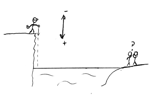

Identify the variables you know and the variable(s) you’re trying to find. Pick a formula that best fits the problem scenario and solve for the unknown.

The rock is released from rest so $ \vec v_i = 0 $. Based on the information given and our sign convention, we can state the following:

(69)¶\[\begin{equation} \vec v_i = 0 \\ \vec a = +9.81 \ m/s \\ t = 1.62\ s \\ \vec d_y = \ ? \\ \vec v_f = \ ? \\ \end{equation}\]

We have 3 known variables and 2 unknown variables in the problem. However, in this case we’re looking for $ \vec d_y $ so we don’t care what $ \vec v_f $ is. If we take a look at the 5 vertical component equations, we see that the following equation has the 3 variables we know and the one we’re looking for:

(70)¶\[\begin{equation} \vec d_y = \vec v_i t + \frac12\ \vec a t^2 \\ \end{equation}\]

We don’t want one with $ \vec v_f $ because we don’t know its value. Using this equation we can solve for $ \vec d_y $:

(71)¶\[\begin{equation} \vec d_y = (0)(2.62\ s) + \frac12\ (+9.81\ m/s^2) (1.62\ s)^2 \\ \vec d_y = +12.8727\ m \\ \vec d_y = +12.9\ m \\ \end{equation}\]

Using the time it took to fell, we can conclude that the cliff is 12.9 meters tall.

Horizontal Component¶

There is no force acting horizontally. Therefore there is no acceleration so it is uniform motion ($ \vec v_i = \vec v_f = \vec v_x $).

Horizontal uniform motion is governed by 3 variables: velocity, range (distance travelled horizontally), and time.

(72)¶\[\begin{equation} \vec v_x , \vec d_x , t \end{equation}\]

These 3 variables are related by the uniform motion equation:

(73)¶\[\begin{equation} \vec v_x = \frac {\vec d_x}{t} \end{equation}\]

Let’s do some practice to solidify the concepts.

__Question 2__

You’re back at the same pond as Question 1 except this time you flick the rock horizontally off the top of the cliff at 30.0 km/h. The rock makes it across the pond and still takes 1.62 seconds to hit the water. How long is the pond?

__Solution__
1) Draw a picture of the scenario. This will give you a better grasp of the problem. 2) Define your sign convention. Assign positive and negative directions to x.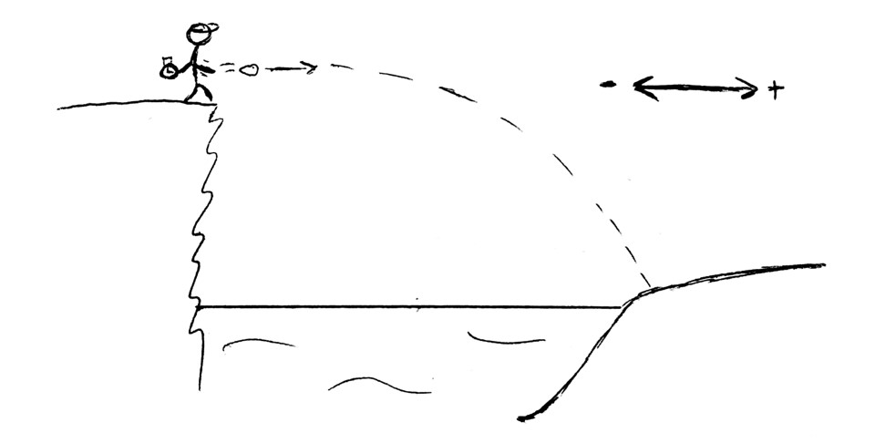

Identify the variables you know and the variable(s) you’re trying to find. Pick a formula that best fits the problem scenario and solve for the unknown.

The horizontal component is easier than the vertical component because there's only one equation with 3 variables. List the 2 variables you know and the one you're trying to find:

(74)¶\[\begin{equation} \vec v_x = +30.0\ km/h =\ +8.3333\ m/s \\ t = 1.62\ s \\ \vec d_x = \ ? \\ \end{equation}\]

Rearrange the uniform motion equation for the unknown and solve:

(75)¶\[\begin{equation} \vec v_x = \frac {\vec d_x}{t} \\ \vec d_x = \vec v_x t = (+8.3333\ m/s)(1.62\ s) \\ \vec d_x = +13.5\ m \\ \end{equation}\]

The pond is 13.5 meters long.

__Question 3__

Evil Knievel, the daredevil stunt driver, is performing his next trick. He speeds horizontally off of a 50.0 m high cliff on a motorcycle. How fast must he leave the cliff-top if he needs to soar over the 90.0 m river at the base of the cliff?

__Solution__
1) Draw a picture of the scenario. This will give you a better grasp of the problem. 2) Define your sign convention. Assign positive and negative directions to both x and y.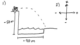

Set up a table and identify the variables you know and the variable(s) you’re trying to find. Pick a vertical component formula that best fits the problem scenario and solve for the unknown.

Based on the information given and our sign convention, we can fill our data table with the following:

\begin{array}{cc} x &y \ \hline \vec d_x = +90.0\ m &\vec d_y = -50.0\ m \ \vec v_x =\ ? &\vec a = -9.81\ m/s^2 \ \ &\vec v_i = 0 \ \end{array} $$ t =\ ? $$

Note that $ \vec v_i = 0 $ because the projectile is launched horizontally, and $ t $ is common to both x & y.

To find $ \vec v_x $, we need $ \vec d_x $ and $ t $. We know $ \vec d_x $ but we’re missing $ t $ so we’ll need to use the vertical data to solve for $ t $. Because we know $ \vec d_y, \vec a, $ and $ \vec v_i $, and we’re looking for $ t $, we’ll use the following equation because we can solve for $ t $ using the variables we know:

(76)¶\[\begin{equation} \vec d = \vec v_i t + \frac12\ \vec a t^2 \\ \end{equation}\]

Because $ \vec v_i = 0 $, the first term goes to 0 and the resulting equation can be rearranged to solve for $ t $:

(77)¶\[\begin{equation} \vec d = \frac12\ \vec a t^2 \\ t = \sqrt{\frac{2 \vec d_y}{\vec a}} \\ \end{equation}\]

Plug in values to find $ t $:

(78)¶\[\begin{equation} t = \sqrt{\frac{2 (-50.0\ m)}{(-9.81\ m/s^2)}} = 3.1928\ s \end{equation}\]

Now that $ t $ is known we can solve for $ \vec v_x $ using the uniform motion equation:

(79)¶\[\begin{equation} \vec v_x = \frac {\vec d_x}{t} = \frac {(+90.0\ m)}{(3.1928\ s)} = +28.2\ m/s \ \ (+101.5\ km/h) \end{equation}\]

__Question 4__

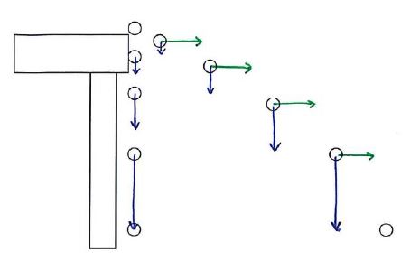
Galileo predicted that an object launched horizontally and an object dropped vertically off the same ledge will reach the ground at the same time. Will they? Why or why not?

__Solution__

Yes, they will. Horizontal and vertical motion are independent for a projectile so the horizontal movement of the launched object does not affect its vertical freefall.

(Drawing courtesy of Ms. Reichelt)

Projectiles Fired at an Angle¶

What happens when your projectile is launched at an angle? What are the initial velocities?

In this case, the initial vertical velocity is no longer 0. It will have some value $ \vec v_i $ that will gradually decrease to 0 at the top of its trajectory and then increase in the downward direction as it returns back to ground. Let’s take a football punt for example.

According to Angelo Armenti’s The Physics of Sports, top-level football kickers can send footballs flying at 70 mph (31 m/s)! If the player kicked it at an angle of 50°, the trajectory would look something like this:

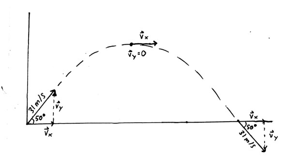
The horizontal velocity $ \vec v_x $ will remain the same throughout the flight (uniform motion) while $ \vec v_y $ will decrease to the top of its trajectory and then increase downwards. Note: If the initial launch height and final landing height are the same ($ \vec d_y $ = 0), then the projectile will land with the same initial speed and angle! The initial horizontal and vertical velocities can be solved with some simple trigonometry:

\[\begin{split} \begin{array}{cc} x &y \\ cos(50^{\circ}) = \frac{adj}{hyp} = \frac{\vec v_x}{31\ m/s} &sin(50^{\circ}) = \frac{opp}{hyp} = \frac{\vec v_y}{31\ m/s} \\ \vec v_x = (31\ m/s)\ cos(50^{\circ}) &\vec v_y = (31\ m/s)\ sin(50^{\circ}) \\ \vec v_x = +19.9264\ m/s &\vec v_y = +23.7474\ m/s \\ \vec v_x = +20\ m/s &\vec v_y = +24\ m/s \\ \end{array} \end{split}\]

__Question 5__

A football player kicks a ball across a flat field at 31.0 m/s and 50.0° from the ground. Find:
a) The maximum height reached
b) The flight time (time before it hits the ground)
c) The range (how far away it hits the ground)
d) The velocity vector at its maximum height
e) The acceleration vector at its maximum height
f) The velocity of the football when it hits the ground

Again, try solving these questions on your own first, it’s the best way to develop your skills. Once you’ve given it a go, click the dropdown arrow to reveal the solution.

__Solution__
__a)__

To find the max height, let's only look at the first half of the flight path. That way, we know $ \vec v_f = 0 $ because projectiles have no vertical velocity at the top of their flight path.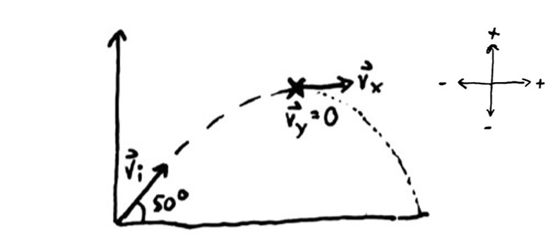

We’ll use the same sign convention from Question 3. Because we’re using the same values from the previous scenario, we can set up our table with the following information:

\begin{array}{cc} x &y \ \hline \vec v_x =\ +19.9264\ m/s &\vec v_i = +23.7474\ m/s \ \ &\vec v_f = 0 \ \ &\vec a = -9.81\ m/s^2 \ \ &\vec d_y =\ ? \ \end{array} $$ t =\ ? $$

Looking at our table, we have 3 knowns and 1 unknown in the vertical column. That means we can solve for $ \vec d_y $. Looking at our vertical component equations, the one that contains our 3 known variables and $ \vec d_y $ is:

(80)¶\[\begin{equation} v_f^2 = v_i^2 + 2 a d \end{equation}\]

$ \vec v_f = 0 $ so we can rearrange and solve for $ \vec d_y $:

(81)¶\[\begin{equation} \vec d_y = -\frac{\vec v_i^2}{2 \vec a} = -\frac{(+23.7474\ m/s)^2}{2\ (-9.81\ m/s^2)} \\ \vec d_y = +28.7431\ m \\ \vec d_y = +28.7\ m \\ \end{equation}\]

b)

To find the flight time, we could either find the time it takes to reach the top of its trajectory and double that, or we could look at the full flight path and find the time to landing. In this case we will choose the latter.

Because our flight path changed, some of our variable have too. In particular, $ \vec d_y = 0 $ which also means that $ \vec v_f = -\vec v_i $. Let’s make a new table:

\begin{array}{cc} x &y \ \hline \vec v_x =\ +19.9264\ m/s &\vec v_i = +23.7474\ m/s \ \ &\vec v_f = -23.7474\ m/s \ \ &\vec a = -9.81\ m/s^2 \ \ &\vec d_y =\ 0 \ \end{array} $$ t =\ ? $$

Now, we’re looking for $ t $ but we don’t have enough horizontal data to solve with uniform motion. However, we know 4 out of the 5 vertical variables which means we have lots of options for the vertical equation. Any of the first 4 equations will do but the second and third will require solving a quadratic equation. To make life easy, we’ll use the first one:

(82)¶\[\begin{equation} \vec a_{ave} = \frac{\vec v_f - \vec v_i}{t} \end{equation}\]

Rearrange and solve for $ t $ (Remember to keep your sign convention. If you don’t you could end up with 0 here!):

(83)¶\[\begin{equation} t = \frac{\vec v_f - \vec v_i}{\vec a_{ave}} = \frac{(-23.7474\ m/s) - (+23.7474\ m/s)}{(-9.81\ m/s^2)} \\ t = 4.8415\ s \\ t = 4.84\ s \end{equation}\]

c)

Now that we have the flight time and $ \vec v_x $, we can use the uniform motion equation to solve for range:

(84)¶\[\begin{equation} \vec v_x = \frac {\vec d_x}{t} \\ \vec d_x = \vec v_x \ t = (+19.9264\ m/s)\ (4.8415\ s) = +96.4730\ m \\ \vec d_x = +96.5\ m \end{equation}\]

d)

At max height, the vertical velocity $ \vec v_y = 0 $ so the only velocity is horizontal.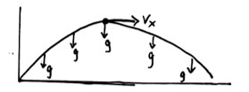

e)

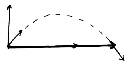
The only acceleration is the acceleration due to gravity which is a constant pointing downwards (see part d for image).

f)

Because $ \vec d_y = 0 $ for the full flight path, $ \vec v_f = -\vec v_i = -23.7474\ m/s $. Horizontal velocity is constant so:

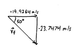(85)¶\[\begin{equation} \vec v_f = 31.0\ m/s\ \ at -50.0^{\circ} \end{equation}\]

__----- Continue on only after attempting Question 5. -----__

"""
If this block of code has suddenly popped up, don't worry! You've found the code 
used to create the Projectile Trajectory graph shown below. This is normally hidden but feel
free to explore it and see how it works.

If you want to hide it again, just click on this code block and press 'Ctrl' and 'Enter' 
simultaneously on your keyboard.
"""


# Import required packages
import numpy as np
import matplotlib as mpl
import matplotlib.pyplot as plt
from ipywidgets import interact
import ipywidgets as widgets
from IPython.display import HTML

# Set values for equations
g = 9.81
t = np.linspace(0,10,100)

# Define equations that plot will display
def d_x(t, theta, v_i):
    return v_i*np.cos(np.deg2rad(theta))*t

def d_y(t, theta, v_i):
    return v_i*np.sin(np.deg2rad(theta))*t - 0.5*g*t**2

# Define options for plot
def f(theta,v_i):
    plt.plot(d_x(t, theta, v_i),d_y(t, theta, v_i))
    plt.ylim(0,50)
    plt.xlim(0,100)
    plt.xlabel("Range (m)", fontsize=16)
    plt.ylabel("Altitude (m)", fontsize=16)
    plt.margins(0)
    plt.grid()
    plt.title("Projectile Trajectory", fontsize=20)
    

hide_me = ''
HTML('''<script>
code_show=true; 
function code_toggle() {
  if (code_show) {
    $('div.input').each(function(id) {
      el = $(this).find('.cm-variable:first');
      if (id == 0 || el.text() == 'hide_me') {
        $(this).hide();
      }
    });
    $('div.output_prompt').css('opacity', 0);
  } else {
    $('div.input').each(function(id) {
      $(this).show();
    });
    $('div.output_prompt').css('opacity', 1);
  }
  code_show = !code_show
} 
$( document ).ready(code_toggle);
</script>
<form action="javascript:code_toggle()"><input style="opacity:0" type="submit" value="Click here to toggle on/off the raw code."></form>''')

The scenario in Question 5 can be modelled by a graph using Python. The following code block creates an interactive graph where you can modify the initial velocity $ \vec v_i $ and launch angle $ \theta $ to see how the projectile’s trajectory changes.

Modify theta and v_i to recreate the scenario in Question 5 and use the graph to verify your answers for Parts (a) and (c) line up.

interact(f,theta = (0,90,5), v_i = (0,31,1));

Pretty cool, huh? If you want to learn how to make graphs using Python, Part (b) of Question 6 will give you a step-by-step breakdown on how to make simple static graphs.

Determining the Optimum Launch Angle¶

__Question 6__

Picture this: The International Olympic Committee runs a worldwide survey to see what new global event people would like to see. After some fierce debate and tallying the votes, shot-cannon is chosen! Shot-cannon is a fairly straightforward sport: each country develops their own medieval cannon that competes in a series of challenges. While each challenge tests a different aspect of the design, the main event is the range competition to see which country’s cannon can fire a lead ball the farthest across the field. Canada has chosen you to man the cannon for the main event! With the cannon already designed and providing a fixed initial velocity $ \vec v_i $, your responsibility is to pick the optimal angle $ \theta $ to fire the cannon to achieve maximum distance. If you assume no air resistance and a flat field, what angle should you pick?

Before reading on, take a moment to picture the scenario in your head and, using your intuition, take a guess at what angle you think would provide the maximum range. Can you think of a way to prove this?

Initially, this problem can seem daunting in its magnitude, but if we break it into two chunks it becomes more manageable:
a) Develop an equation for the range $ \vec d_x $ as a function of $ \vec v_i $ and $\theta $. That is, come up with an equation in the form of $ \vec d_x = f(\ \vec v_i,\ \theta)$.
b) Determine the optimal angle from the equation you’ve developed.

Part (a) can be solved using the skills you’ve just learnt so give it a go and hit the arrow to check your answer.
Part (b) can be solved with coding and graphing which will be covered in the next section Python Basics.

__Solution__
__a)__

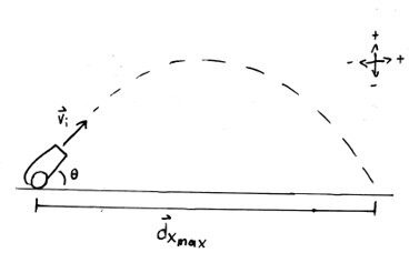
With a picture and sign convention drawn, let’s mark down the values we know in a table. While we don’t know the angle $\theta$, and $ \vec v_i $ is an unknown constant, we can still write down $ \vec v_x $ and $ \vec v_{i_y} $ in terms of $\theta$ and $ \vec v_i $ because we ultimately want an equation with these terms:

\begin{array}{cc} x &y \ cos(\theta) = \frac{adj}{hyp} = \frac{\vec v_x}{\vec v_i} &sin(\theta) = \frac{opp}{hyp} = \frac{\vec v_y}{\vec v_i} \ \vec v_x = \vec v_i cos(\theta) &\vec v_y = \vec v_i sin(\theta) \ \vec v_x = v_i cos(\theta) &\vec v_y = v_i sin(\theta) \ \end{array}

The vector arrow on $ v_i $ is dropped because we know it’s positive in both directions based on our sign convention. Also, we assume a flat field so $ \vec d_y = 0 $ which means that $ \vec v_{y_f} = -\vec v_{y_i} $ Therefore, our data table becomes:

\begin{array}{cc} x &y \ \hline \vec v_x =v_i cos(\theta) &\vec v_i = v_i sin(\theta) \ \vec d_x =\ ? &\vec v_f = -v_i sin(\theta) \ \ &\vec a = -g \ \ &\vec d_y =\ 0 \ \end{array} $$ t =\ ? $$

Acceleration is written as $ -g = -9.81 m/s^2 $ for simplicity. Note that this is a constant written as a letter, not a variable.

In order to come up with an equation for $ \vec d_x $, we first need an equation for $ t $ in terms of the given variables $ \vec v_i $ and $\theta$. Considering we know or have expressions for 4 of the vertical values, we will choose the first equation which makes it easy to solve for t:

(86)¶\[\begin{equation} \vec a_{ave} = \frac{\vec v_f - \vec v_i}{t} \end{equation}\]

Rearrange and solve for $ t $:

(87)¶\[\begin{equation} t = \frac{\vec v_f - \vec v_i}{\vec a_{ave}} = \frac{(-v_i sin(\theta)) - (v_i sin(\theta))}{(-g)} \\ t = \frac{2 v_i sin(\theta)}{g} \\ \end{equation}\]

This expression can be applied to the horizontal component to come up with an equation for $ \vec d_x $:

(88)¶\[\begin{equation} \vec v_x = \frac{\vec d_x}{t} \\ \vec d_x = \vec v_x t \\ \vec d_x = (v_i cos(\theta)) (\frac{2 v_i sin(\theta)}{g}) \\ \vec d_x = \frac{2}{g} v_i^2 sin(\theta) cos(\theta) \\ \end{equation}\]

Knowing that $ g $ and $ v_i $ are constants, this means that $ \vec d_x $ is only a function of the variable $\theta$.

__----- Continue on only after attempting Question 6 Part (a) and checking with the solution. The next section will cover Part (b). -----__

Python Basics¶

From this point on, there are two ways to solve for $\theta$: you can use calculus to solve for it analytically, or we can get creative and use coding with graphing to find the answer!

Python provides us with some great tools to graph this function easily. If you have some knowledge of Python you can skip the explanations and just run the code cells. If not, we’re going to take a moment to understand what the code you’re about to see does. First up, let’s go over the first bit of code.

Imports
At the beginning of most Python programs you’re more than likely to see a few (or many) import statements. The purpose of these is to bring in other pieces of code, that either you or someone else have written, in order to keep your current program more manageable. For example, the set of import statements we’re going to use to plot our functions look like this (click on the code block below and press Ctrl and Enter on your keyboard simultaneously to run the cell).

%matplotlib inline
import matplotlib
import numpy as np
import matplotlib.pyplot as plt

Starting from the top down, let’s go over what each piece of this code does.

%matplotlib inline: This is very specific to the Jupyter notebook we’re using. This tells matplotlib (next bullet) to output graphs in the cell directly below the one in which the code is executed. For more information about Jupyter “magic commands” feel free to read this document.
import matplotlib: This command tells Python to import the matplotlib package. This package contains the python functions that we’ll be using for plotting.
import numpy as np: This imports the python package numpy or “numerical python” and assigns the name to it within our code to np so we don’t have to type out numpy every time we need a function. We’ll be using this package for mathematical functions like sine and the square root.
import matplotlib.pyplot as plt: This imports the graphing subroutines from the matplotlib packages and assigns them the name plt so we don’t have to type as much when we want to produce a graph.

Plotting
After required modules have been imported into our script, we’re ready to get started graphing. First up, we need to define a number of points which to plot. Our computer doesn’t understand that the variable $ \theta $ is fully continuous, so we have to give it a discrete set of points to plot our function with. We can do that in python using numpy as follows (click the next cell and press control and enter at the same time on your keyboard).

theta = np.linspace(0,90,5)
print("theta = ", theta)

theta =  [ 0.  22.5 45.  67.5 90. ]

This creates a list of numbers called theta which consists of 5 numbers evenly spaced in the domain $[0,90]$ that we’ll use to plot our function. The print function is a standard python function that simply displays our variables to the screen as either numbers or characters. In order to plot our functions, we type the following. Note that we’ve increased the number of points in theta to create a smoother plot. Feel free to change the number 100 to something smaller and observe how the plot changes. We also assigned a value to v_i and g so that the computer can plot the function numerically. Likewise, play around with these numbers and see how your range changes.

theta = np.linspace(0,90,100)
v_i = 30.0
g = 9.81
plt.plot(theta, 2 / g * (v_i**2) * np.sin(np.deg2rad(theta)) * np.cos(np.deg2rad(theta)))
plt.show()

../../../_images/projectile-motion_31_0.png

There’s a fair bit going on in that last line of code that should be noted. First, by using plt.plot we’re calling a function from matplotlib.pyplot (that we called plt) called plot. This function, unsurprisingly, is used to tell Python what to plot. We then pass this function a number of arguments (AKA inputs). The first argument theta is the list of numbers we generated earlier. The second argument 2 / g * (v_i**2) * np.sin(np.deg2rad(theta)) * np.cos(np.deg2rad(theta)) is the mathematical function we’re going to plot. Here theta is the variable we’re going to plot, and also the list of points that we generated earlier. The ** is the Python way of saying “to the power of”. Because sin and cos functions take radians as an input and not degrees, we use np.deg2rad which is a function that converts degrees to radians.

So, what we’re really saying here is “plot $ \frac{2}{g}v_i^2 \sin(\theta)\cos(\theta) $ for 100 $\theta$ values between 0 and 90”.

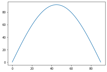
Now, that graph is missing a lot of important things like axis labels and a legend. We can add those like this:

plt.plot(theta, 2 / g * (v_i**2) * np.sin(np.deg2rad(theta)) * np.cos(np.deg2rad(theta)))
plt.xlabel(r"$ \theta (deg) $", fontsize=16)
plt.ylabel(r"$ \vec d_x (m) $", fontsize=16)
plt.margins(0)
plt.grid()
plt.title(r"Range as a function of launch angle $ \theta $")
plt.show()

../../../_images/projectile-motion_33_0.png

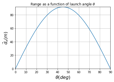
where the plt. calls are still calling functions from matplotlib.pyplot however this time we’re creating x axes labels with plt.xlabel and y axes labels with plt.ylabel. plt.margins(0) removes any unnecessary blank space around the graph and plt.grid() adds a nice grid to visually locate points on the graph easier. Finally, plt.title adds a title bar to our graph. The dollar signs and “r” characters are just there to make the lettering look nice. Play around with the code and see if you can change the title bar, label font sizes, and margins.

Based on the plot above, we see that the maximum range lines up with a launch angle of 45° . Was this your initial guess?

With no air resistance, 45° is the optimal angle because it provides the best compromise between horizontal speed and height. If you shoot it below 45°, you’ll get a faster horizontal velocity but the ball will also hit the ground quicker because there’s less flight time. If you shoot it above 45°, you’ll get more flight time but a slower horizontal velocity. 45° is the sweet spot between extremes.

Because the graphical solution takes the shape of a parabola, this also demonstrates an important symmetry in the launch angles. Launch angles that are equidistant from the maximum of 45° will have the same range. That is, 30° and 60° have the same range, 15° and 75° have the same range, etc. The wonders of physics!

3. Conclusion & Extension¶

This notebook has demonstrated the basics of projectile motion that can be used to determine flight paths, speeds, and times. Reasoning for why projectile motion is foundational to physics is explained, followed by a breakdown describing the horizontal and vertical components of projectile motion. The two components were brought together in an angled launch example with an interactive graph and the final question utilized Python programming to solve a basic calculus problem. Applying the skills taught in this notebook to your practice examples will give you a strong grasp of projectile motion analysis and enable you to begin designing your own basic launchers!

Practice: Projectile Game¶

For a great interactive visualization of projectile motion, check out the PhET link below!

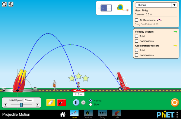
Click to Run

Callysto Curriculum Notebooks