
Module 3 Unit 2 - Importing Data Sets#
While we looked at a number of different data structures in the last units, a lot of the data sets used in data science are organized as two-dimensional arrays—like a spreadsheet or table with multiple rows and columns.
Because of this, our focus will be on ways to create DataFrames from data sets.
Adding data to a DataFrame#
There are lots of ways to add data to DataFrames. Which method is best for a project depends on how much data there is and where we are getting it from.
Three common methods we’ll explore are:
Creating the DataFrame by hand inside a Jupyter notebook—for small data sets
Loading the DataFrame from a file in the Jupyter notebook—for small to medium data sets
Loading the DataFrame from an online resource—useful for large data sets or when accessing secondary data sets from online repositories or open data portals, such as Stats Canada or The Global Health Observatory
Creating a DataFrame by hand#
Get the most out of this section by opening a Jupyter notebook in another window and following along. Code snippets provided in the course can be pasted directly into your Jupyter notebook. Review Module 2, Unit 5 for a refresher on creating and opening Jupyter notebooks in Callysto.
As we saw earlier in the course, DataFrames organize data into rows and columns.
For small data sets, like our table of Canadian coins less than a dollar, we can just type the data points directly into our code by hand. This is similar to what we did in the DataFrame tutorial and activity in Unit 1.
An important step when constructing a DataFrame is creating our dictionary. A dictionary is the code that establishes each column’s header and list of values under that header.
For example, in the code below we recreate our coins_df DataFrame.
import pandas as pdfrom pandas import DataFrame
data = {'name': ['penny', 'nickel', 'dime', 'quarter'],
 'value': [1, 5, 10, 25],
 'weight': [2.35, 3.95, 1.75, 4.4],
 'design': ['Maple Leaves', 'Beaver', 'Schooner', 'Caribou'] }
DataFrame(data)
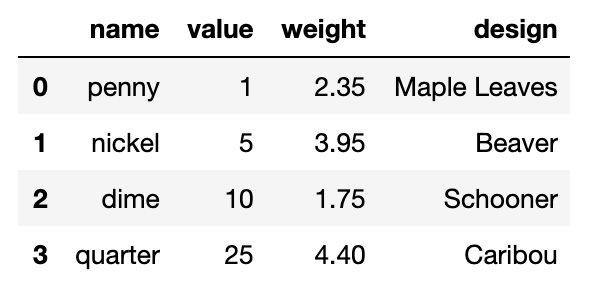
A demonstration of how to show the output of a completed DataFrame, using Python programming. The Python programming used to show the completed DataFrame about the penny, nickel, dime, and quarter was “coins_df.”
The output is a DataFrame which holds all the data in a nicely organized format.
The far-left column is the DataFrame’s row index, and by default is a column of numbers counting up from 0. However we can also make one of the columns we created the row index instead by adding the following line to our Jupyter notebook:
DataFrame(data,index=['a','b','c','d'])
So, if you need to quickly analyze a small amount of data, it’s easy to just type in the data directly into the Jupyter notebook. For larger amounts of data, you might need to transfer data in another format directly into a DataFrame.
For example, another way to create a DataFrame from data stored in code is to start with a numerical array, such as we might get from Numerical Python or NumPy.
🏷️ Key Term: NumPy#
Numerical Python (NumPy) is a library of code functions and data structures that are useful for a wide variety of numerical calculations. NumPy is widely used for scientific computations in Python.
We can convert a two-dimensional (2D) array directly into a DataFrame by passing the array code to DataFrame, like this:
#

A demonstration of how to assign numerical values in a DataFrame through “Numerican Python.” This Python programming function is also called “NumPy.”
🏷️ Key Term: Array#
An array is 2D when the values are organized into rows and columns, like a table on a 2D piece of paper. It’s also possible for arrays to be 1D arrays and even 3D arrays, however we won’t be exploring those in this course.
As we can see, the column headers and row index are numbers. To make the DataFrame more readable, we can establish labels for them by including a definition in our code.
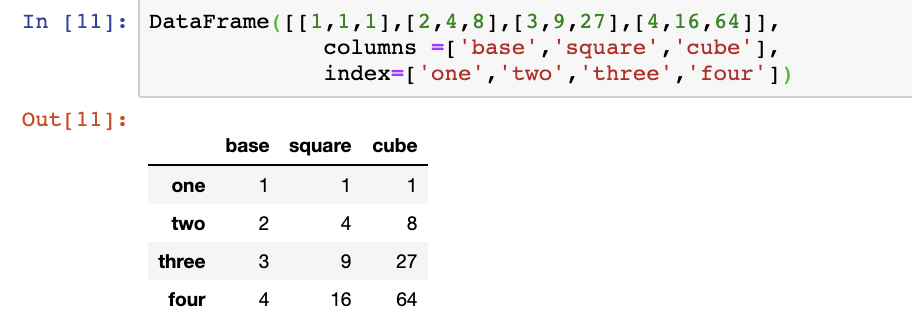
A demonstration of how to create a pandas dataframe using arrays, and how to assign desired column names, as well as row index names. In this case, each array represents one row. Four arrays denote four columns. Each array is of size three. Correspondingly we add three column names: ‘base’, ‘square’, ‘cube’ and four row names ‘one’, ‘two’, ‘three’, ‘four’.
2D NumPy arrays aren’t the only data structures that can be converted into a DataFrame. Others include:
A 2D NumPy Masked array of numbers (which includes masked values)
A dict of arrays, lists, or tuples (each dict item becomes a column)
A dict of Series, or a dict of dicts
A list of Series, or a list of dicts
A list of lists, or a list of tuples
Another DataFrame
When converting another data structure into a DataFrame, the syntax of our code will be the same as when we converted our 2D NumPy array.
The syntax is the same as above, in code like this line:
array_df = DataFrame(myData)
where myData is one of the above data structures (array, dict, list, etc) and array_df is the DataFrame that is created from that data.
Creating DataFrames by hand works well for small amounts of data. However, it would get more difficult to do this by hand with large data sets.
Loading data from a Callysto Hub file#
Many data sets are too big to store directly within the code. Many data sets we’ld work with in a classroom would be stored in another file which is referenced by the code.
Since we’re creating and running our Jupyter notebooks online, any files we wish to use need to also be online. We can make data files available to our Jupyter notebooks by adding them to the Callysto Hub.
This section contains tutorials! Get the most out of them by opening a Jupyter notebook in another window and following along. Code snippets provided in the course can be pasted directly into your Jupyter notebook. For more information about using Jupyter notebooks, review Module 2 Unit 5.
Spreadsheet files (CSV)#
Spreadsheet files, such as those created in Microsoft Excel or other spreadsheet software, are frequently used to collect and store data, and are often saved in a file format like Comma-separated Values (.csv).
We can easily bring data from CSV files in the Callysto Hub into our Jupyter notebook using code.
Let’s try that now.
🏁 Tutorial: Adding CSV data to a DataFrame#
If you have a spreadsheet file on your computer that you’d like to work with in a Jupyter notebook, you’ll need to upload it to the Callysto Hub before you can reference it in your project.

For this tutorial, we’ll use code to generate a new CSV file and use it as our source for the DataFrame.
Step 1
In your Jupyter notebook, run the following code to create a new CSV file in your Callysto Hub.
python%%writefile Colours.csv
Colour,Emotion,Preference,Length
Yellow,Joy,2,3
Blue,Sadness,3,7
Red,Anger,6,5
Purple,Fear,5,4
Green,Disgust,4,7
Black,Grief,7,5
White,Ecstasy,1,7
The %%writefile command will create a new file named Colours.csv that contains a small data set about colour.
Step 2
Next, check the contents of this new file with a !cat command.
!cat Colours.csv
!cat is a handy command for displaying a file’s contents.
The result should look like this.
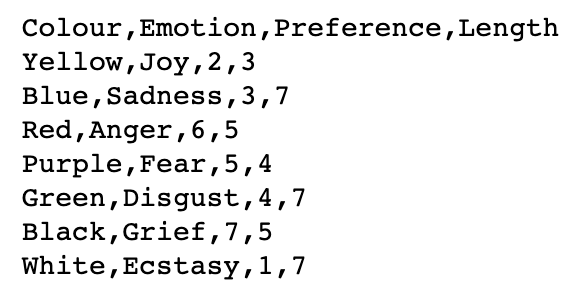
A data set about colours associated to emotions: ‘joy’, ‘sadness’, ‘anger’, ‘fear’, ‘disgust’, ‘grief’, ‘ecstasy’. Dataset is ‘comma-separated’ and has four data categories – colour associated to emotion, emotion, preference towards emotion (on a numerical scale), and length of the word associated to that emotion.
If the data set does not display correctly, try going back to Step 1 and inputting the commands into a new code cell.
Step 3
Now let’s set up our DataFrame.
To access the data in the Colours.csv spreadsheet file, we’ll use the read_csv command, which we’ll import from the pandas library.
Run the code below in your Jupyter notebook.
from pandas import read_csv
colours_df = read_csv('Colours.csv')
colours_df
When using this command, the name of the data file must be surrounded by single quotation marks. Single quotes tells the Jupyter notebook the text refers to a file name, so it knows exactly what to look for. If we omit these quotation marks, the code will give an error when we run it.
We’ll name our new DataFrame colours_df and finish by calling up our DataFrame by name to check that we did it correctly.
The output should look like this:
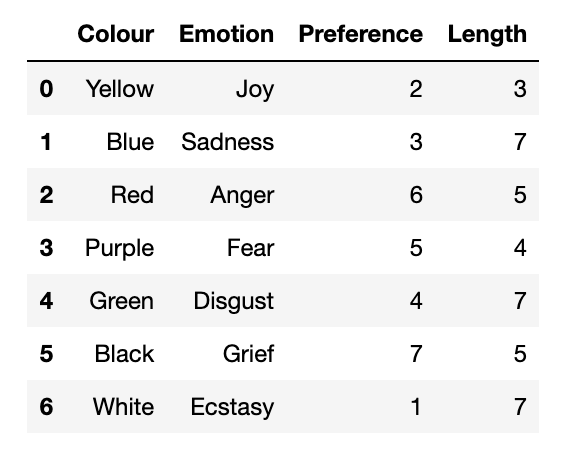
A pandas dataframe containing data on colours associated to emotions: ‘joy’, ‘sadness’, ‘anger’, ‘fear’, ‘disgust’, ‘grief’, ‘ecstasy’. Dataframe has four data columns – colour associated to emotion, emotion, preference towards emotion (on a numerical scale), and length of the word associated to that emotion. Each row is assigned indeces ranging from 0 to 6.
Many data sets we work with will be fairly large, so we may not always want to read in the entire thing. To limit the number of rows in our DataFrame, we can modify the read command. For instance, here we read in only the first 5 rows:
read_csv('Colours.csv',nrows=5)
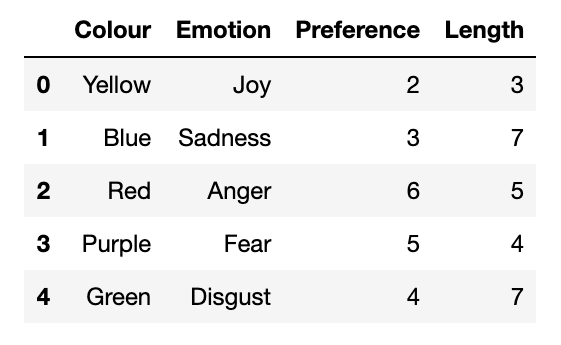
A pandas dataframe containing data on colours associated to emotions: ‘joy’, ‘sadness’, ‘anger’, ‘fear’, ‘disgust’. Dataframe has four data columns – colour associated to emotion, emotion, preference towards emotion (on a numerical scale), and length of the word associated to that emotion. Each row is assigned indeces ranging from 0 to 4.
In practice, data scientists often start by reading in just a few rows so they can try out ideas on a smaller portion of the data set before doing a full analysis.
Text files (TXT)#
Similar to read_csv, there is a command called read_table which can locate a table of data stored within a simple text file and load that data into a DataFrame. It works best with text files of the .txt type.
read_table is pretty flexible, and is able to do this even when the table is formatted using tabs or different numbers of spaces.
For example, a text file that looked like this:
C1 C2 C3
R1 123 45 67
R2 12 345 678
R3 11 222 22
could be read in with this line of code:
read_table('file.txt',sep='\s+')
The option sep=’\s+’ tells the Jupyter notebook that the numbers in the file are separated by various amounts of white space, rather than a simple tab or comma.
The read_table command can also be used to access a CSV as well, since a CSV is essentially a table separated by commas:
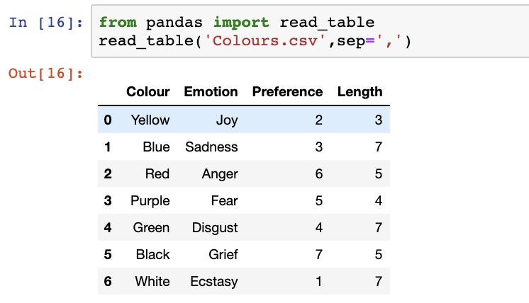
Python code needed to read the dataset on emotions and transform it into a pandas dataframe. The read_table function is imported from the pandas library. Then the read_table function is used, passing the name of the dataset ‘Colours.csv’ along with a separating value ‘,’ - recall our dataset is comma-separated. This is specified using sep=’,’.
If you have a text file with tables of data, try using read_table. You can read about the various options available to read in most common table formats.
In a pinch, though, you could always use a spreadsheet program to turn the table into a CSV file, and load that in directly.
Loading data from an online resource#
From online files#
Many governments, companies, and organizations provide data publicly available in the form of downloadable files or Application Programming Interfaces (APIs).
As we’ve seen, spreadsheet and text files can be added to our Callysto Hub. However if a file is already online, another way is to simply reference the file from the place where we found it.
This not only saves us a step, but also ensures we’re accessing the most current version of the data. When the organization providing the information updates the file, we’ll see those changes reflected in our project.
Let’s try that now.
🏁 Tutorial: Adding data from a file on a website#
For this tutorial, we will use a CSV about pet adoptions created by the folks at www.bootstrapworld.org.
The file is not in the Callysto Hub, and we won’t be adding it. Instead, we’ll use code to reference it directly from the website where it is hosted.
In a Jupyter notebook, run the code below:
from pandas import read_csv
url = "https://tinyurl.com/y917axtz-pets"
pets = read_csv(url)
pets
We can see that these lines of code perform the following tasks:
Import the read_csv command from pandas
Specify the url we’ll be accessing the file from
Name our new DataFrame pets
Call up the DataFrame to ensure we created it correctly
The output should look like this:
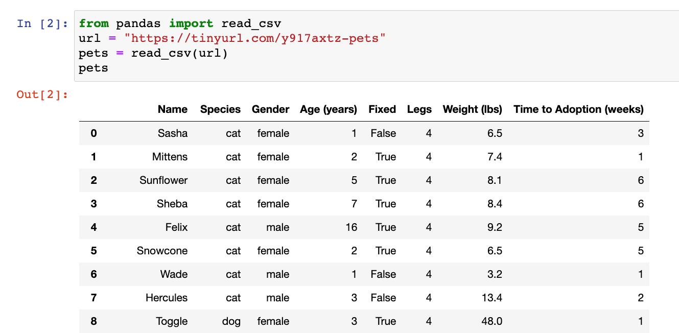 A pandas DataFrame resulting from Python programming being used to read a data set about pet adoption.
Loading data from an online resource#
From a website#
🏁 Tutorial: Grabbing data from tables on a website#
For this tutorial, we’ll access a Wikipedia page that has several tables about baseball statistics. The webpage is here: https://en.wikipedia.org/wiki/Baseball_statistics
The pandas library has a handy tool for pulling all the tables directly from the website where it’s hosted.
In a Jupyter notebook, run the code below:
from pandas import read_html
url = 'https://en.wikipedia.org/wiki/Baseball_statistics'
df_list = read_html(url)
df_list[3]
We can see that these lines of code perform the following tasks:
Import the read_html command from pandas
Specify the url we’ll be accessing the file from
Name our list of DataFrames df_list
Call up one of the DataFrames in the list to see what is there
The output should look like this:
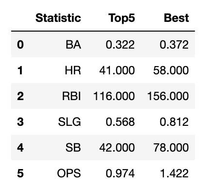
*A pandas DataFrame loaded from https://en.wikipedia.org/wiki/Baseball_statistics. *
In fact, there are several DataFrames in this list. You may like to read through them all, by examining df_list[0], df_list[1], df_list[2], and so on.
From website APIs#
An API is an application programming interface (API). It is a set of software tools that can be included in a website to allow code written by other people to interact with that website.
When an open data portal has an API available, we have direct access to the data from the Jupyter notebook. From there, we can load the data into a DataFrame for immediate use.
This method is a little more advanced, so we won’t be exploring API use in this course. However, experienced programmers are encouraged to look into how different portal APIs work.
When a web page or web server has an API available, there’s usually an FAQ on the web page explaining in detail how to use it. Different websites can have different APIs, so always read the FAQ!
Three important Python libraries that are used to access data through APIs are:
pandas, which provides the DataFrame construction for us
requests, which allows us to send HTTP requests, which handles the calls to the company’s website
json, which manages JavaScript Object Notation for us
There are three basic steps:
Send a get request to the website where the data we want can be accessed. This makes the data available to our Jupyter notebook.
Convert the data to a standard Python format (we’re using JSON).
Create a new DataFrame from our JSON-format data.
🏁 Explore (Optional)#
This Jupyter notebook is the first in a series of four notebooks on 1) Socrata and the SODA API, 2) Plotly, 3) joining datasets, and 4) filtering datasets.
Conclusion#
In this section, we discussed getting data into a data structure known as a DataFrame. Once we have the data saved in a DataFrame, it becomes easy to access individual pieces of data in the DataFrame and start doing our data analysis. The next unit discusses how to use a DataFrame once the data is in it.

