Module 3 Unit 4 - Cleaning and Filtering Data Sets

This section contains tutorials! Get the most out of them by opening a Jupyter notebook in another window and following along. Code snippets provided in the course can be pasted directly into your Jupyter notebook. Review Module 2, Unit 5 for a refresher on creating and opening Jupyter notebooks in Callysto.

The more accurate and representative our data set is, the more useful it is for data analysis. However, data sets often come with errors — mistakes made by people collecting or entering data, or caused by computer glitches when saving, copying, or transmitting data.

When doing data science, it’s always a good idea to review our data and filter out faulty observations.

In this unit, we’ll explore ways to:

• Select and view particular data in a DataFrame

• Add and remove rows

• Reorder rows

• Modify values

• Replace values

• Find outliers

The activities in this unit use a coin_df DataFrame similar to the one we created earlier in the course.

Create coin_df by running the code below.

from pandas import DataFrame
data = {'name': ['penny', 'nickel', 'dime', 'quarter'],
 'value': [1, 5, 10, 25],
 'weight': [2.35, 3.95, 1.75, 4.4],
 'design': ['Maple Leaves', 'Beaver', 'Schooner', 'Caribou'] }
coin_df = DataFrame( data )
coin_df

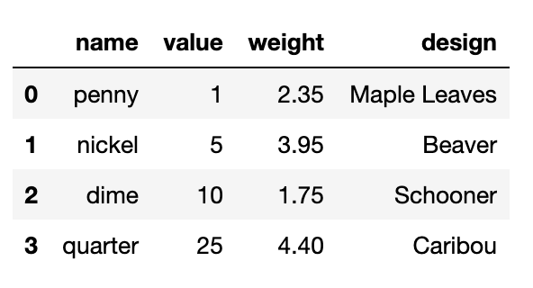
A demonstration of how to show the output of a completed DataFrame, using Python programming. The Python programming used to show the completed DataFrame about the penny, nickel, dime, and quarter was “coins_df.”

🏁 Activity: Common functions

This table provides some common functions and what they look like as a line of code. Try each one out and see what kind of output they produce.

Operation	Description
coin_df['name']	Select (and print out) a column
coin_df[['name','weight']]	Select two columns
coin_df.loc[1]	Select a row
coin_df.loc[1,'name']	Select a single value in row/column
coin_df.loc[1,'name'] = 'NICKEL'	Change a single data point in row/column
coin_df[coin_df['weight']>3]	Select all the rows where the weight of the coin is greater than 3

Adding another row to the DataFrame

If we want to expand our data set, we can use the loc command to add a new row and specify its index and values. Let’s try that now.

Run the code below in your Jupyter notebook to add another row to the coin_df DataFrame.

coin_df.loc[4] = ['50-cent piece', 50, 6.9, 'Coat of Arms']
coin_df

The outcome should look something like this:

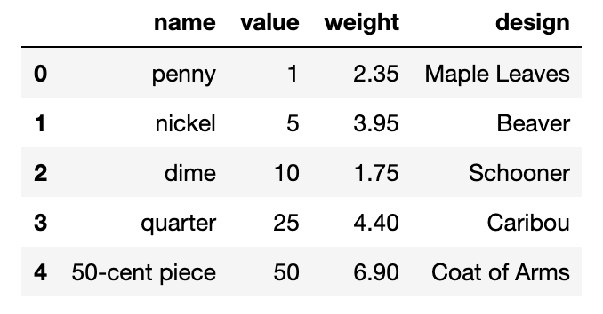
A DataFrame containing data on the value, weight and design of various coins. The first five include ‘penny’, ‘nickel’, ‘dime’, ‘quarter’, ‘50-cent piece’. Each row contains information for each of these coins.

In this example, we set the row index for the new coin to be 4, but when adding a row we can actually set it as nearly any unused rational number. For example, we could make the row index 7, 42, 5000, -71, or 3.14592 (pi to the 5th decimal).

Dropping a row from the DataFrame

Conversely, if we want to remove some data from our DataFrame, we can use the drop function. For instance, the following line of code will remove the row with index 0.

coin_df.drop(index=0)

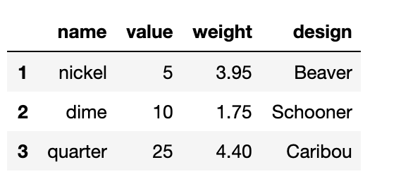
A DataFrame containing data on the value, weight and design of various coins after the ‘penny’ row has been removed. The first three include ‘nickel’, ‘dime’, ‘quarter’. Each row contains information for each of these coins.

Notice that this is actually a new DataFrame with one fewer row than the DataFrame coin_df. If you want to change coin_df itself, use the inplace option:

coin_df.drop(index=0, inplace=True)

Reordering rows in the DataFrame

Sometimes it’s helpful to order rows in a data set according to the data, rather than their default row index number. For example, we might want to display our coin data in alphabetical order.

The reindex function lets us specify a particular row order.

coin_df.reindex([2,1,0,3])

Try this in your own notebook now. The outcome should look like this:

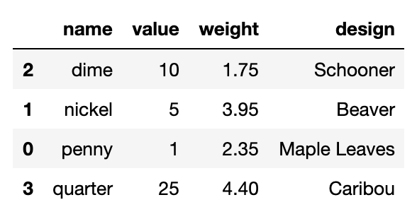
Demonstration of sorting coins DataFrame by name, using alphabetical order. Order of rows changes to reflect: data for dime, then data for nickel, then data for penny, then data for quarter. Note that data for 50-cent piece does not appear here.

Modifying values in the DataFrame

Earlier in the course, we explored how to modify an entire column of entries at once by applying a simple mathematical formula, similar to this one:

coin_df['value'] = coin_df['value']/100
coin_df

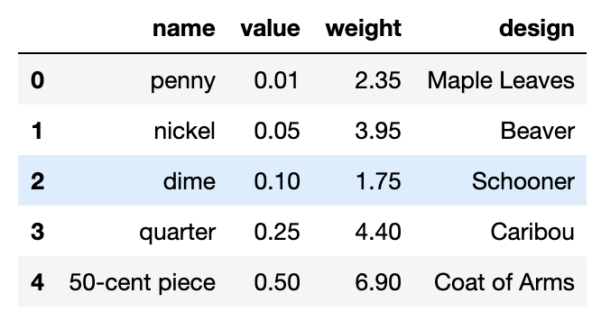
Demonstration of sorting coins DataFrame by weight, in ascending order. The lowest value is 0.01 corresponding to penny, followed by 0.05 corresponding to nickel, followed by 0.10 corresponding to dime, followed by 0.25 corresponding to quarter, followed by 0.50 corresponding to 50-cent piece.

This method is good for a bulk modification to numbers, but what if we want to modify text values, also known as strings?

🏷️ Key Term: String

In Python, a string is a specific sequence of characters. Any value in a data set that is not a number is a string, such as a name or label.

For this we can use the map command.

For example, right now all the text in our DataFrame is lowercase — except for the values under the design column. The following command shows what the text looks like in lower case.

coin_df['design'].map(str.lower)

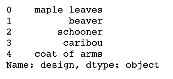
Demonstration of turning all words under the desing column into lower case. Sorted by value. Printed on screen: 0 (row index) maple leaves, 1 (row index) beaver, 2 (row index) schooner, 3 (row index) caribou, 4 (row index) coat of arms. Name of column: design. Type object.

Remember, this doesn’t change the original DataFrame, it just outputs the result. If you are happy with this result, then you can store it back in the DataFrame, like this:

coin_df['design'] = coin_df['design'].map(str.lower)

Lambda functions (Optional)

Lambda functions allow us to use a function as a parameter to another function, like the map function mentioned earlier in the course.

For instance, suppose we needed a function that would let us double all the weight values in our data set.

We could start by defining a function called Doubler and pass it to the map function, like this:

def Doubler(x):
    return x+x
coin_df['weight'].map(Doubler)

However, a more succinct way is to represent the Doubler function in the call to map, like this:

coin_df['weight'].map(lambda x: x+x)

So this way, the Doubler function is represented in the map function as a parameter, using the form of a lambda notation.

We call this type of function an anonymous function, because we never define it with a specific name.

In a more useful example, we might like to specify a numerical function that converts units for the weights.

The lambda function defined via the statement:

lambda x : x*28.35

will convert ounces to grams. We can apply this to the weight column, with the map function calling up the lambda function:

Demonstration of changing the value under weight column for each column using lambda functions. Using the .map() method we can change the weight that appears for each column as follows coins_df[‘weight’].map(lambda x: x28.35). This will multiply each value under the ‘weight’ column by 28.35.*

Practice this yourself with this code:

coin_df['weight'].map(lambda x: x*28.35)

Replacing values

If a value in our DataFrame isn’t quite right, we can replace it with a new one.

For example, the design on a Canadian dime shows a schooner sailing ship. However, most people know it represents a racing ship built in Halifax, Nova Scotia, in the 1920s – the Bluenose.

The Bluenose photographed in 1921 by W. R. MacAskill

Let’s use the replace function to make the design entry for the dime display as the more familiar Bluenose.

coin_df['design'].replace('Schooner','Bluenose')

Demonstration of replacing the word “Schooner” for “Bluenose” under the desing column in coin_df. This can be done as follows coin_df[‘design’].replace(‘Schooner’,’Bluenose’).

This function is particularly useful when there are multiple instances of a word that needs to be replaced.

For example, if we wanted to change the word cat to feline in the pets DataFrame we created earlier in the course.

🏁 Activity: ?

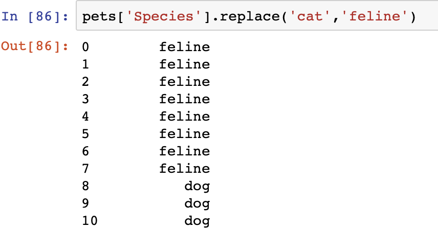Demonstration of replacing the word “cat” for “feline” under the Species column in pets. This can be done as follows: pets[‘Species’].replace(‘cat’, ‘feline’).

The replace function can be applied to both numbers and text.

A common use is to replace a marker value in a data set, like -999, with the more useful np.nan designation from the NumPy library.

pets['Legs'].replace(-999,np.nan)

🏷️ Key Term: Marker Value

A marker value indicates that something unusual happened when a specific data point was recorded. For example, if a researcher’s equipment broke, there might not be data for a specific day. Rather than leaving the entry blank for that day, they might use a clearly identifiable value like -999 to indicate the data point isn’t available. We shouldn’t use that value in any calculation of averages or minimum temperatures, so it should be replaced before doing any analysis.

🏷️ Key Term: Not a Number (NaN)

Numerical Python, or Numpy, has a special value to represent a data point that is Not A Number or briefly NaN. Rather than storing a special value like -999 to indicate missing data, a NaN indicates no number was recorded here. Python and pandas are smart enough to know that they should not use NaNs in their calculations of averages, maximum values, plotting the data, etc. So they are very handy placeholders for data in a programming environment.

Finding Outliers

One way we can find errors is by looking for values that seem unusually high or low compared to the rest of the data set — outliers.

Many of the mathematical functions we’ve already explored can help us find and examine outliers in our data.

For example, we could use the min and max functions to identify the lowest or highest values in a column.

Demonstration of computing the maximum age of pets. Using the notation pets[‘Age (years)’].max() we can obtain the maximum age of pets from the pets DataFrame.

Or, use a mathematical formula to display all the rows with a value that falls below or above a particular threshold.

Demonstration of subsetting the pets dataframe by the Age column: selecting pets older than 8 years. Subsetting occurs in two stages: first select values under ‘Age (years)’ column satisfying the condition ‘older than 8 years’. We can do that via the command pets[‘Age (years)’] >8. The second stage is obtaining all column values for pets older than 8 years old. We can do so as follows pets[pets[‘Age (years)’] >8].

DataFrames come with idxmax and idxmin functions, which output the index number for the row with the highest or lowest value in the specified column.

Demonstration of idxmax(), idxmin() to return index of first occurrence of max and min, pet Age. pets[‘Age (years)’].idxmax() returns the index where the max age is found. Correspondingly pets[‘Age (years)’].idxmin() returns the index where the min age is found.

Once we know the index for a row, we can easily view it to learn more about the data in that row, and decide if it seems reasonable.

Demonstration of how to access the 5th row on the pets DataFrame (we start counting from 0). We can use the loc property to access a the information associated to a row number. In Python we start counting from 0, so that the first row has index 0, second row index 1, …, fifth row has index 4. To use this code, call pets.loc[4] to return values associated to each column for pet in fifth row.

🏁 Activity:

Using your Jupyter notebook, find the pet that took the longest to adopt. Is there anything interesting about this pet?

Also check, which pet had the most legs? What kind of animal is it?

Other methods for cleaning and organizing data

There are many other methods for finding and addressing errors in DataFrames beyond what we have explored in this unit.

As you become more comfortable using DataFrames in Jupyter notebooks, we encourage you to explore the resource below for more information about what they can do.

Explore

This reference page provides an overview of the essential functionality common to the pandas data structures. Essential basic functionality

This reference page provides an overview of the essential functionality common to the pandas data structures.

Conclusion

So far we’ve seen a variety of techniques for manipulating quantitative data in a DataFrame, like counts and measurements.

In the next unit, we’ll explore methods for manipulating qualitative data, like names, labels, and descriptions.