Module 3 Unit 3 - Working with DataFrames

Once we have a DataFrame set up in a Jupyter notebook, we want to be able to explore it. Many data sets are too large to take in all one time, or might be so big they take our computer time to process. To reduce the time and impact on our computer to process data, we have methods to look at specific sections or summaries of the data.

In this unit, we’ll explore how to:

• View the head of the DataFrame—a snapshot of just the first few rows

• Access a specific column, row, or value in a DataFrame

• Make updates to the DataFrame

• Perform calculations using the values in the DataFrame

• Create a simple graph from the DataFrame

These are by no means the only ways to work with DataFrames, but they’re a good place to start.

The activities in this unit use the pets DataFrame we created earlier in the course. If you need to recreate it, follow the steps below.

This section contains tutorials! Get the most out of them by opening a Jupyter notebook in another window and following along. Code snippets provided in the course can be pasted directly into your Jupyter notebook. Review Module 2, Unit 5 for a refresher on creating and opening Jupyter notebooks in Callysto.

🏁 Tutorial: Creating the pets example DataFrame

Step 1

Import the functions you need. For this tutorial, we’ll need the DataFrame function and the read_csv function from pandas.

from pandas import DataFrame, read_csv

Step 2

The data is coming from a CSV file hosted on a website, so we need to tell our Jupyter notebook the url where the data is located.

url = "https://tinyurl.com/y917axtz-pets"

Step 3

We also specify a name for our DataFrame (pets) and call up the DataFrame to check that we created it correctly.

pets = read_csv(url)
pets

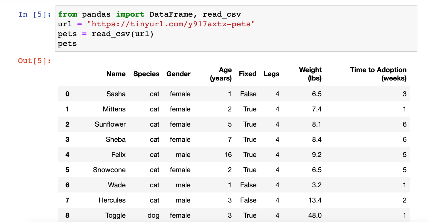
The output should look something like this:

From the pandas Python library, the functions DataFrame and read_csv are imported. A CSV (comma-separated-value) dataset containing data on pet adoption is stored in a URL. The function read_csv() can be used to read the content of that dataset and store it as a pandas DataFrame in a variable called ‘pets’.

Viewing the head of a DataFrame

Typically, the DataFrame contains a lot of values and it’s not always practical to read in the entire thing when we want to check something.

It’s often useful to look at just the first few rows of data. For this, we use the head function. Here’s how it works:

Data on pet adoption has been stored into a pandas DataFrame using the read_csv() function. The DataFrame is stored in a variable called ‘pets’. To access the first five rows, we use the .head() method. Applied as pets.head()

pets is the name of the object we created, and head is a function that reveals the first few rows of data.

🏁 Activity: Running the head function in your Jupyter notebook

pets.head()

The result should like this:

First five rows of a DataFrame containing data on pet adoption. DataFrame contains eight columns with information about each pet: ‘Name’, ‘Species’, ‘Gender’, ‘Age’ (in years), ‘Fixed’, ‘Legs’, ‘Weight’ (in lbs), and ‘Time to Adoption’ (in weeks). Each row corresponds to one pet, and the rows contain complete information for each of the columns.

The head function defaults to revealing just five rows of data. Can you figure out how to specify the number of rows you want to reveal?

Accessing a specific column, row, or value

Data sets might have many rows and columns, more than can easily be navigated when viewing all the data at once.

We can generate a list of all the column headers in our data set using the column function, like this:

pets.columns

Here’s how it works:

Demonstration of how to access the column names of the DataFrame using the ‘columns’ property. To access the column names of the ‘pets’ DataFrame, we use the notation pets.columns. The column names are returned: ‘Name’, ‘Species’, ‘Gender’, ‘Age (years)’, ‘Fixed’, ‘Legs’, ‘Weight (lbs)’, ‘Time to Adoption (weeks)’.

Now that we can see all the columns available in the DataFrame, we can pick out a specific one to examine.

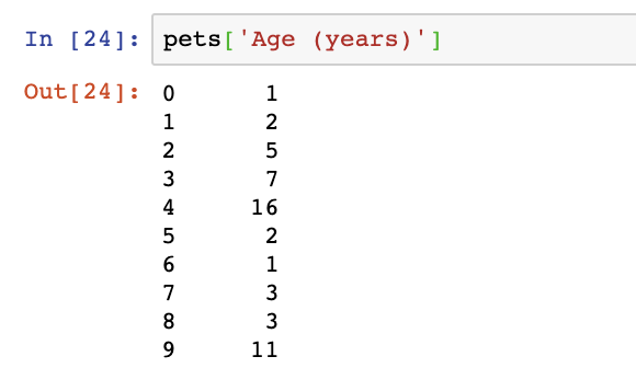
The heading Age (years), looks interesting. Let’s access our pets DataFrame again and display just this one column, which we select using the square brackets notation on the pets DataFrame:

pets['Age (years)']

Demonstraton of how to access the values under the column ‘Age (years)’. In Python, square brackets [ ] are used to access the values under a column. The notation used is name_of_dataframe[‘Column_name’]. In this example, to access the age of the different pets, the notation used it pets[‘Age (years)’], which returns the index number of each row (starting from 0, increasing by one each row) on the left hand side, and the age of the pet on the right hand side. So pet on index 0 is 1 year old, pet on index 1 is 2 years old, pet on index 2 is 5 years old, so on.

Now let’s try pulling the values in a single row. For this, we’ll use the loc (location) function.

The row index for our pets DataFrame is numbered, so to view a single row we’ll need the number associated with that row.

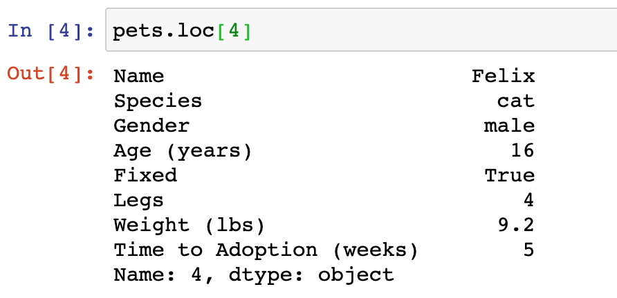
We can see above that one of the animals in our DataFrame is 16 years old, which is the oldest in our data set! Let’s look at the rest of the data for that animal by viewing row 4.

pets.loc[4]

Demonstration of how to access the 5th row on the pets DataFrame (we start counting from 0). We can use the loc property to access a the information associated to a row number. In Python we start counting from 0, so that the first row has index 0, second row index 1, …, fifth row has index 4. To use this code, call pets.loc[4] to return values associated to each column for pet in fifth row.

We can also use the loc function to pull a single data point from our data set, by selecting both the row and column.

pets.loc[3,'Name']

Demonstration of how to access the Name of the pet in fourth row. Using pets.loc[3,’Name’], we can access the name of the pet on the fourth row.

Correcting or changing data

Sometimes, we may need to correct or update our data set. Changes we make in the code do not affect the original data source—the CSV file we’re pulling our pets data from is not being altered. Instead, the code is manipulating how the data appears to us inside our Jupyter notebook.

For example, if we wanted the full name of the Sheba in row 3 to appear in the name column, we could do this:

pets.loc[3,'Name']='Queen of Sheba'
pets.head()

From the pandas Python library, the functions DataFrame and read_csv are imported. A CSV (comma-separated-value) dataset containing data on pet adoption is stored in a URL. The function read_csv() can be used to read the content of that dataset and store it as a pandas DataFrame in a variable called ‘pets’.

We can also change an entire column to display differently.

For example, we could convert the weight values from pounds (lbs) to kilograms (kg).

Let’s try that now.

🏁 Tutorial: Converting a column of values from pounds to kilograms

Step 1

In your Jupyter notebook with the pets DataFrame set up, run this code to multiply all the values in the Weight column by 0.4536 to convert them from lbs to kg:

pets['Weight (lbs)']=0.4536*pets['Weight (lbs)']
pets.head()

The head command in the last line will pull up the first 5 rows of the data set, so we can confirm the change worked.

The output should look similar to this:

Demonstration of how to change the values of a column: transforming Weight (lbs) to Weight (kg).

Step 2

Now, we need to update the header of the column to reflect the new unit of measurement.

Use the rename function to update the weight column header.

pets.rename(columns = {'Weight (lbs)':'Weight (kg)'},inplace=True)
pets.head()

The output should look like this:

Demonstration of how to change the name of a column with new values ‘Weight (lbs)’ to ‘Weight (kg)’.

Did you notice the first line included an option inplace=True? This option tells our Jupyter notebook that we are updating the existing pets DataFrame, and not creating a new one with a different column name.

Computing with the data

With mathematical functions we can begin to perform calculations and do some simple analysis.

For example, we can determine the range of ages present in our data set, and calculate the average age of all the pets.

Demonstration of how to print minimum, maximum and average values for a given column. Using the .min(), .max(), and .mean() methods, we can print, respectively, the minimum, maximum and average values for the age of the pets via the following notation: Minimum age of pets: pets[‘Age (years)’].min(). Maximum age of pets: pets[‘Age (years)’].max(). Average age of pets: pets[‘Age (years)’].mean()

These are just like the functions we saw earlier with the Series object. We used a print command so we can print out all three numbers together.

Here is a list of commonly used functions that help with statistical data analysis.

Function	Description
min(), max()	The minimum and maximum values in the list
numpy.argmin(), numpy.argmax()	The location in the list, where the minimum or maximum occurs
mean(), median()	Mean is the arithmetic average, median is the middle value in the ordered list of values
numpy.var(), numpy.std()	Variance and standard deviation, a measure of how spread out the data is
pd.DataFrame.skew(), pd.DataFrame.kurt()	Skew and kurtosis, another measure of the spread of the data
sum()	The sum of all values in the list
numpy.cumsum()	The incremental, cumulative sum of values in the list
numpy.prod(), numpy.cumprod()	The product of values, and the incremental, cumulative product of values
numpy.diff()	The arithmetic difference of adjacent pairs of values in the list—often used for time series to notice changes in data in a list
pd.DataFrame.pct_change()	The percentage difference between adjacent change in pairs of values in the list

🏁 Activity: Computing the minimum and maximum values

In your Jupyter notebook, compute the minimum and maximum values in the Times to Adoption column.

pets.head()

Also compute the mean and median. Are the mean and median values close, or not?

Revealed Code:

print(
pets['Time to Adoption (weeks)'].min(),
pets['Time to Adoption (weeks)'].max(),
pets['Time to Adoption (weeks)'].mean())

Creating simple graphs from a DataFrame

Graphs are a type of data visualization, which we’ll explore in much more detail later in the course.

For now, let’s try creating a simple graph from our pets DataFrame.

The DataFrame data structure actually has a built-in plot function that lets us create some simple visualizations.

To use this function, we specify what kind of plot we are creating, which column from our DataFrame will be the x-axis, and which column will be the y-axis.

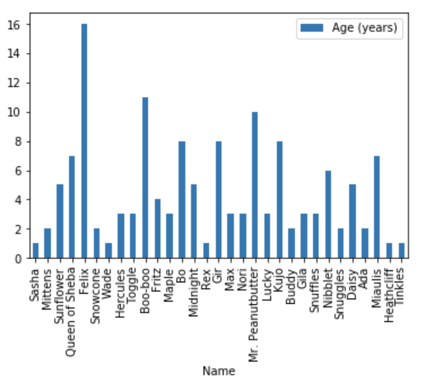
pets.plot(kind='bar', x='Name', y='Age (years)');

The output should look something like this:

Demonstration of how to print minimum, maximum and average values for a given column. On the x axis we see the name of each pet, and on the y axis we see the age (in years). The oldest pet is Felix, who is 16 years old.

🏁 Activity: Discussion

We often hear that older animals are adopted at different rates from younger animals. Does our data reflect this?

Create a graph that compares the Time to Adoption and the Age (years) of the animals in our data set.

What does the plot tell you about who gets adopted quicker?

Conclusion

In this unit, we showed how to access data inside a DataFrame, modify that data, add more information to the DataFrame, and begin some calculations on the data. We also showed how to plot data from the DataFrame, which is our first step towards creating powerful data visualization.

The next unit will address more complex ways to manipulate data in a DataFrame which are useful when cleaning and filtering our data.