Analyzing Radical Functions¶

Mathematics 20-2¶

from IPython.display import display, Math, Latex, HTML, clear_output, Markdown
import numpy as np
import matplotlib.pyplot as plt
from numpy import sqrt as sqrt
import ipywidgets
from ipywidgets import widgets, interact, interactive, interact_manual, Button, Layout

%matplotlib inline

Introduction¶

This notebook will explain how to analyze and graph radical functions. We will look at the square root function, which is the most common type of radical, as well as other forms of radicals.

The most important thing to understand about radical functions is where the function exists. This is often called the domain of existence and will be further explained in the notebook. Looking at rational functions will incorporate aspects of intervals and inequalities. It will also help find the roots of quadratic equations.

Background¶

Radical Functions¶

A radical function is any function that is inside a radical. This tells us that some function, \(f(x)\), is contained within a fractional exponent. This can be written as:

\[f(g(x)) = g(x)^{\frac{1}{n}}\]

Where \(n\) is an integer for the following exercises.

So what does \(g(x)\) look like? Well, it can take on any form! Let’s look at a few examples of different \(g(x)\) functions:

If \(g(x) = x\), then \(f(g(x)) = g(x)^{\frac{1}{n}} = x^{\frac{1}{n}}\)
If \(g(x) = x^2 + 2x\), then \(f(g(x)) = (x^2 + 2x)^{\frac{1}{n}}\)
If \(g(x) = \frac{x^3 - 9x + 3}{2x - 1}\), then \(f(g(x)) = \Big(\frac{x^3 - 9x + 3}{2x - 1}\Big)^{\frac{1}{n}}\)

The most common radical function is the square root function:

\[\sqrt{x}\]

Which is equivalent to writing:

\[x^{\frac{1}{2}}\]

So if we wanted to obtain the square root of some function \(f(x)\), this is done by doing:

\[\big[ \ f(x) \ \big]^{\frac{1}{2}} = \sqrt{f(x)}\]

Now, if we try finding the root of a function, (where \(f(x) = 0\)), understanding how radicals work becomes important. If we only look at quadratic functions of the form:

\[f(x) = ax^2 + bx + c\]

There are many cases where the roots of this function can be found immediately by taking the square root. But, remember that when you take the square root of a single value, such as \(4\), we get the result of:

\[\sqrt{4} = \pm \ 2\]

Where either positive, (\(+\)), or negative, (\(-\)), \(2\) can be squared to produce a value of \(4\):

\[(2)^2 = (-2)^2 = 4\]

This exact same principle applies when dealing with functions. For example, let us look at the function \(f(x) = x^2\):

# function to be plotted
x = np.linspace(-10,10,100) 
fx = x**2.

# plot showing f(x) = x^2 with (2,4) and (-2,4) plotted points to show +/- result for square roots.
plt.figure(1,figsize = (10,7))
hold = True
ticks = np.arange(-5,6)

plt.plot(x,fx,'r-',label = r'$f(x) = x^2$')
plt.plot([-10,10],[0,0],'k-',alpha = 1,linewidth = 1)
plt.plot([0,0],[-10,15],'k-',alpha = 1,linewidth = 1)
plt.plot(2,4,'k.',markersize = 10)
plt.plot(-2,4,'k.', markersize = 10)
plt.grid(alpha = 0.7)
plt.legend(loc = 'lower right',fontsize = 13)
plt.xticks(ticks)
plt.ylim([-2,15])
plt.xlim([-5,5])
plt.show()

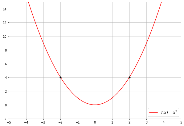
../../../_images/analyzing-radical-functions_8_0.png

As you can see, at both \(x=2\) and \(x = -2\) our function equals \(4\), which is marked with the black dots.

If you were to take the square root of this function \(f(x) = x^2\) you could write it as the following:

\[\sqrt{f(x)} = \sqrt{x^2} = (x^{2})^{\frac{1}{2}}\]

Where you may be tempted to write the final answer like this:

\[\sqrt{x^2} = \pm \ x\]

This is the formatting we had for a single value like \(4\). But, when taking the square root of a function, \(\pm\) doesn’t actually tell you what is happening in this scenario. Instead, we write it as:

\[\sqrt{x^2} = \lvert x \rvert\]

Where \(\lvert x \rvert\) is defined as the absolute value function. This means that:

If \(x \geq 0\), then \(\lvert x\rvert\) equals \((x)\)
If \(x < 0\), then \(\lvert x\rvert\) equals \(-(x)\)

Our second line states that “If \(x<0\), then \(\lvert x \rvert\) equals \(-(x)\)”. This means that for any negative value of \(x\), we substitute that value into the \(x\) in \(-(x)\), and get a double negative. This results in a positive value. For example: \(\lvert -2 \rvert = -(-2) = 2\). This is true for all negative values inside the absolute value function.

A formal definition of this would be:

\[\begin{split}\lvert x\rvert = \begin{cases}x , & \text{if } x\geq 0 \\ -(x),& \text{if }x<0\end{cases}\end{split}\]

Now that we’ve introduced the absolute value function, we can begin finding the roots of some quadratic functions.

Remember that the root of a function is where \(f(x) = 0\). In our initial example, where \(f(x) = x^2\), we can prove by inspection of our graphic that the function has a root at \(x = 0\). But, if we were to find this function’s root more rigorously, you would follow these steps:

Set \(f(x)\) equal to \(0\) so that \(f(x) = x^2 = 0\).
Take the square root of BOTH sides so that \(\lvert x \rvert = 0\)
Solve the expression for the POSITIVE case of the absolute value function.

For step 3 we only look at the positive case of the absolute function. This is because, in our formal definition, the only condition where \(x\) is defined at 0 is when x is positive. This is what is needed to solve for the root.

How about a less trivial example?

Let’s look at the function:

\[h(x) = x^2 - 10x + 25\]

If you can, take a moment to try and factor this by hand. You should end up with an expression that looks like \((x-a)^2\), where \(a\) is an integer value. To check your answer, click on the button below.

#Construction of button to provide factored polynomial result.
buttonShowAnswer = widgets.Button(description="Show Answer")

def displayAnswer(a):
    display(Math('x^2 - 10x + 25 = (x-5)^2'))
    buttonShowAnswer.close()

display(buttonShowAnswer)
buttonShowAnswer.on_click(displayAnswer)

This is in the same form as our last example, since \((x-5)\) is all squared. Therefore, we can follow the exact same steps as before:

\(\sqrt{(x-5)^2} = 0\)
\(\lvert(x-5)\rvert = 0\)
Positive case: \(x-5 = 0\) \(\color{red}\rightarrow\) \(x=5\)

We’ve found the root!

It is important to note that functions of the form \(f(x) = (ax-b)^2\) only have 1 real root. This root can be found by inspecting the graph or by applying the method we just saw.

So what would all these operations look like graphically? This is a good opportunity to practice making graphs of mathematical functions in Python!

First off, let’s look at our original functions \(f(x)\) and \(h(x)\). Graphically, the \(x\) value is in the range of \([-5,10]\), (We are only looking at the values of \(x\) between \(-5\) and \(10\), including \(-5\) and \(10\)).

# functions to be plotted
x = np.linspace(-10,10,1000)
fx = x**2.
gx = (x-5)**2.

# plot showing f(x) and g(x)
plt.figure(1,figsize = (10,7))
hold = True
plt.plot(x,fx,'r-',label = r'$f(x) = x^2$')
plt.plot(x,gx,'b-',label = r'$g(x) = (x-5)^2$')
plt.plot([-10,10],[0,0],'k-',alpha = 1,linewidth = 1)
plt.plot([0,0],[-10,10],'k-',alpha = 1,linewidth = 1)
plt.grid(alpha = 0.7)
plt.legend(loc = 'lower right',fontsize = 13)
plt.xticks(np.arange(-5,11))
plt.ylim([-2,5])
plt.xlim([-5,10])
plt.show()

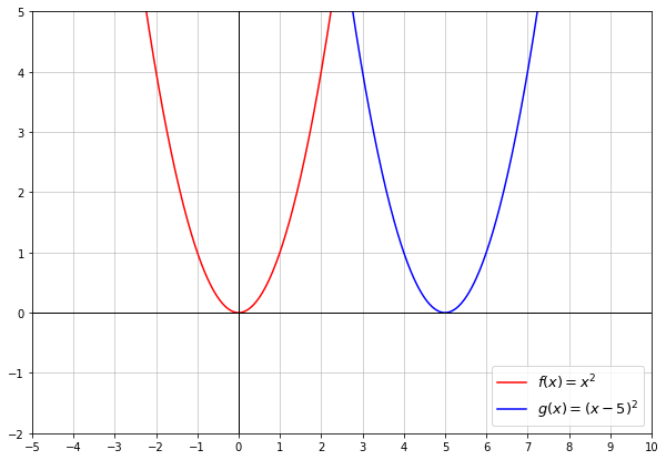
../../../_images/analyzing-radical-functions_14_0.png

As we found earlier, \(f(x)\) and \(h(x)\) are parabolas with roots at \(x = 0\) and \(x = 5\) respectively.

The next step will be to take the square root of our functions and check what this process looks like. This time, you will input the required code for the functions, so that you become familiar with how to do it. To do this, here’s a quick overview of how you type mathematical symbols:

\(+\) and \(-\) are simply typed as you see here
To do multiplication (\(\times\)), you must type in an asterisk, ( \(^{*}\) )
To do division (\(\div\)), you must type in a forward slash, ( \(/\) )
To do an exponent (\(x^{n}\)), you must type in two asterisks followed by the exponent, ( \(x^{**}n\) )
To do a square root (\(\sqrt{x}\)), you must type “\(sqrt(x)\)”.

from IPython.display import clear_output
x = np.linspace(-10,10,1000)

#Used to ensure the description text doesn't get cut off.
style = {'description_width': 'initial'}

#Create an input text widget.
question = widgets.Text(
    value=None,
    description='Type your answer here: ',
    disabled=False,
    style = style
    )

#Create a button titled "Check Answer"
checkButton = widgets.Button(description = "Check Answer")

def checkAnswer(a):
    #questionAnswer will be the input given by the user.
    questionAnswer = question.value
    
    #answers is a list of possible answers that can be inputted. 
    answers = ["sqrt((x-5)**2)", "(x-5)", "x-5"]
    
    #Check if the input is in the list of answers. If this is the case:
    if questionAnswer in answers:
        clear_output()
        display(writtenQuestion)
        print("You answered: " + questionAnswer)
        print("Well done!")
        
        fx = sqrt(x**2)
        gx = sqrt((x-5)**2)
        
        # plot the absolute value functions of both f(x) and g(x)
        plt.figure(1,figsize = (10,7))
        hold = True
        plt.plot(x,x**2.,'r-',label = r'$x^2$')
        plt.plot(x,fx,'m--',label = r'$\sqrt{x^2}$')
        plt.plot(x,(x-5)**2.,'b-',label = r'$(x-5)^2$')
        plt.plot(x,gx,'c--',label = r'$\sqrt{(x-5)^2}$')
        plt.plot([-10,10],[0,0],'k-',alpha = 1,linewidth = 1)
        plt.plot([0,0],[-10,10],'k-',alpha = 1,linewidth = 1)
        plt.grid(alpha = 0.7)
        plt.legend(loc = 'lower right',fontsize = 13)
        plt.xticks(np.arange(-5,11))
        plt.ylim([-2,5])
        plt.xlim([-5,10])
        plt.show()
    
    #Otherwise, if no answer has been given, do nothing.
    elif (questionAnswer == ""):
        None
    
    #Lastly, if the answer is wrong, give the user a hint.
    else:
        clear_output()
        display(writtenQuestion)
        display(question)
        display(checkButton)
        print('Not quite right. \nRemember, the answer is just "sqrt(h(x))"')

#writtenQuestion is the question the user is asked.
writtenQuestion =  Latex(
"Using the syntax from above, please enter what the \
square root of $h(x) = (x-5)^2$ is, (Remember to include brackets)")

displayn(writtenQuestion)
display(question)
display(checkButton)

checkButton.on_click(checkAnswer)

Using the syntax from above, please enter what the square root of \(h(x) = (x-5)^2\) is, (Remember to include brackets)

To summarize, taking the square root of functions of the form:

\(>\)\(f(x) = (ax-b)^2\)

Where \(a\) and \(b\) are constants, will give the result:

\[\sqrt{f(x)} = \lvert ax-b\rvert\]

We can also generalize the principle root, which will be denoted as \(x_0\), of such functions as

\[x_0 = \frac{b}{a}, \qquad a \neq 0 \]

Note¶

Rational Exponents (n \(\geq\) 2)¶

As mentioned before we defined a radical function to be of the form \(f(g(x)) = g(x)^{\frac{1}{n}}\). Now we are going to look at functions where \(n\geq2\).

Below is an interactive slider. Moving the slider will change the value of \(n\) in our rational exponent expression. See what happens when you move this around.

#Construction of interactive plot to visualize x^(1/n)
def slider(n):
    x = np.linspace(1e-7,10,500)
    if n != 0:
        plt.figure(1,figsize = (10,7))
        hold = True
        plt.plot(x,x**(1./n),'b-',linewidth = 2,label = str((r'$y = x^{1/' + str(n) + '}$')))
        plt.xlabel('$x$',fontsize = 14)
        plt.ylabel('$y$',fontsize = 14)
        plt.plot([-10,10],[0,0],'k-',alpha = 1,linewidth = 1)
        plt.plot([0,0],[-10,10],'k-',alpha = 1,linewidth = 1)
        plt.grid(alpha = 0.7)
        plt.xticks(np.arange(-5,11))
        plt.ylim([-2,5])
        plt.xlim([-5,10])
        plt.legend(loc = 'best', fontsize = 18)
        plt.show()

    return n

#Store a slider with a range between 2 and 10 in the character j.
j = interactive(slider, n=(2,10,1))
display(j)

Likewise, we can look at functions where the exponent is negative, such that:

\[f(g(x)) = g(x)^{\frac{-1}{n}} = \frac{1}{g(x)^{\frac{1}{n}}}\]

Again, an interactive graph is shown below, to observe how changing the value of n affects the behaviour of the function.

#Construction of interactive plot to visualize x^(-1/n)
def slider(n):
    x = np.linspace(1e-7,10,500)
    if n != 0:
        plt.figure(1,figsize = (10,7))
        hold = True
        plt.plot(x,x**(1./n),'b-',linewidth = 2,label = str((r'$y = x^{-1/' + str(abs(n)) + '}$')))
        plt.xlabel('$x$',fontsize = 14)
        plt.ylabel('$y$',fontsize = 14)
        plt.plot([-10,10],[0,0],'k-',alpha = 1,linewidth = 1)
        plt.plot([0,0],[-10,10],'k-',alpha = 1,linewidth = 1)
        plt.grid(alpha = 0.7)
        plt.xticks(np.arange(-5,11))
        plt.ylim([-2,5])
        plt.xlim([-5,10])
        plt.legend(loc = 'best', fontsize = 18)
        plt.show()

    return n

#Store a slider with a range between -2 and -10 in the character j.
j = interactive(slider, n=(-10,-2,1))
display(j)

We can see that no matter what value appears in the exponent, the function is always greater than 0.

This is because a radical function like \(x^{\frac{1}{n}}\) is only defined for values of \(x\geq0\). Functions like \(x^{\frac{-1}{n}}\) are also only defined for values of \(x > 0\). This is true of all radical functions. So:

An expression under an exponent \((1/n)\) must be a POSITIVE value
An expressions under an exponent \((-1/n)\) must be both POSITIVE and NON-ZERO

Some examples of this are:

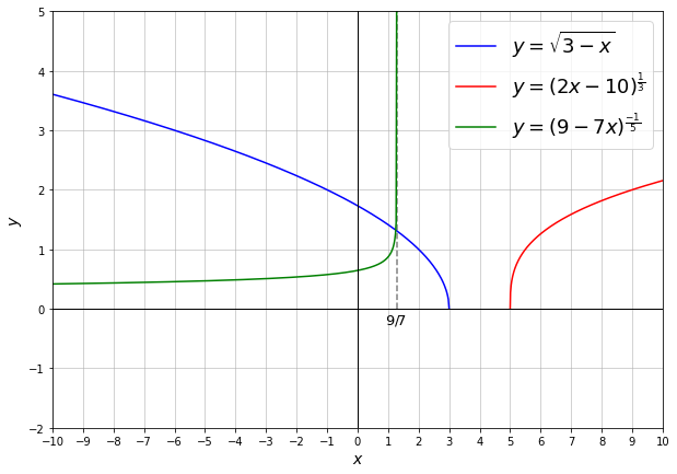
\(\ \sqrt{4-x}\) must be a POSITIVE quantity.
\(\ (2x-10)^{\frac{1}{3}}\) must be a POSITIVE quantity.
\(\ (9-7x)^{\frac{-1}{5}}\) must be a POSITIVE and NON-ZERO quantity.

So what exactly does this mean? How do we know where these quantities become negative? What might these functions look like? This will all be answered in the next section!

Domain of Existence¶

It is very important that the value underneath a fractional exponent (\(\frac{1}{n}\)) is positive. Where the values are positive defines the domain of existence. Let’s see if we can figure out what the domains of existence are for \(a)\), \(b)\) and \(c)\).

For \(a)\), we need to see where \((4-x) \geq 0\). To do this, we can follow these steps:

Write out the expression, ( \((4 - x) \geq 0\) )
Isolate for \(x\), ( \(-x \geq -4 \) )
Ensure that \(x\) doesn’t have a negative sign in front of it, ( \(x \leq 4\) )

Note¶

Remember that flipping a sign from negative, (\(-\)), to positive, (\(+\)), will flip the inequality. This is also true the other way around, (Flipping a sign from positive to negative).

So, we’ve found that the domain of existence for \(\sqrt{4-x}\) is all \(x\) values such that \(x \leq 4\).

Now, \(b)\) and \(c)\) will be left for you to solve and input into the boxes provided below. Remember, we want to find where the expression under the exponent is positive. If you get stuck, look back to how the domain of existence was found for function \(a)\).

How to Input Domain of Existence¶

Let’s say we wanted to input our answer for the domain of existence of \(\sqrt{4-x}\), (Which was \(x \leq 4\)). The input formatting for the “less than or equal to” symbol is written exactly how it is said. So, if you are given an input box to enter your answer, you would type in:

x <= 4

Spaces are important. You should also write fractions like \(\frac{5}{3}\) as “\(5/3\)”

from IPython.display import clear_output

#Used to ensure the description text doesn't get cut off.
style = {'description_width': 'initial'}

#Create an input text widget.
question = widgets.Text(
    value=None,
    description='Input: ',
    disabled=False,
    style = style
    )

checkButton = widgets.Button(description = "Check Answer")

def checkAnswer(a):
    #questionAnswer will be the input given by the user.
    questionAnswer = question.value
    
    #answers is a list of possible answers that can be inputted. 
    answers = ["x <= 4"]
    
    #Check if the input is in the list of answers. If this is the case:
    if questionAnswer in answers:
        clear_output()
        display(writtenQuestion)
        print("You answered: " + questionAnswer)
        print("Well done!")
    
    #Otherwise, if no input has been given, do nothing:
    elif (questionAnswer == ""):
        None
    
    #Lastly, if the answer is wrong, give the user a hint:
    else:
        clear_output()
        display(writtenQuestion)
        display(question)
        display(checkButton)
        print('Not quite right. \nRemember, you only have to type in "x <= 4".')

#writtenQuestion is the question the user is asked.
writtenQuestion =  Latex('Type "$x <= 4$" into the input box below to ensure you are \
using the appropriate syntax.')

display(writtenQuestion)
display(question)
display(checkButton)

checkButton.on_click(checkAnswer)

\[\text{Type} "x <= 4" \text{into the input box below to ensure you are using the appropriate syntax.}\]

from IPython.display import clear_output
#Used to ensure the description text doesn't get cut off.
style = {'description_width': 'initial'}

question = widgets.Text(
    value=None,
    description='Input: ',
    disabled=False,
    style = style
    )

checkButton = widgets.Button(description = "Check Answer")

def checkAnswer(a):
    #questionAnswer will be the input given by the user.
    questionAnswer = question.value
    
    #answers is a list of possible answers that can be inputted. 
    answers = ["x >= 5"]
    
    #Check if the input is in the list of answers. If this is the case:
    if questionAnswer in answers:
        clear_output()
        display(writtenQuestion)
        print("You answered: " + questionAnswer)
        print(correct)
    
    #Otherwise, if no input has been given, do nothing:
    elif (questionAnswer == ""):
        None
    
    #Lastly, if the answer is wrong, give the user a hint:
    else:
        clear_output()
        display(writtenQuestion)
        display(question)
        display(checkButton)
        print(hint)

#writtenQuestion is the question the user is asked.
writtenQuestion =  Latex("Find the domain of existence for: $(2x - 10)^{1/3}$")

#hint is the hint the user is given when the answer is incorrect.
hint = 'Not quite right. \nRemember, the process to find the domain of existence is:\n\
    1. Write out the expression,\n\
    2. Isolate for x, \n\
    3. Ensure that x is not negative.'

#correct is the message outputed for when the user gets the question correct.
correct = "Well done!\n\
    1. Write out the expression, ((2x - 10) >= 0),\n\
    2. Isolate for x, (x >= 5),\n\
    3. Ensure that x doesn't have a negative sign, (x >= 5)"

display(writtenQuestion)
display(question)
display(checkButton)

checkButton.on_click(checkAnswer)

\[\text{Find the domain of existence for: } (2x - 10)^{1/3}\]

from IPython.display import clear_output
#Used to ensure the description text doesn't get cut off.
style = {'description_width': 'initial'}

question = widgets.Text(
    value=None,
    description='Input: ',
    disabled=False,
    style = style
    )

checkButton = widgets.Button(description = "Check Answer")

def checkAnswer(a):
    #questionAnswer will be the input given by the user.
    questionAnswer = question.value
    
    #answers is a list of possible answers that can be inputted. 
    answers = ["x < 9/7", "x < (9/7)"]
    
    #Check if the input is in the list of answers. If this is the case:
    if questionAnswer in answers:
        clear_output()
        display(writtenQuestion)
        print("You answered: " + questionAnswer)
        print(correct)
    
    #Otherwise, if no input has been given, do nothing:
    elif (questionAnswer == ""):
        None
    
    #Lastly, if the answer is wrong, give the user a hint:
    else:
        clear_output()
        display(writtenQuestion)
        display(question)
        display(checkButton)
        print(hint)

#writtenQuestion is the question the user is asked.
writtenQuestion =  Latex("Find the domain of existence for: $(9 - 7x)^{-1/5}$")

#hint is the hint the user is given when the answer is incorrect.
hint = 'Not quite right. \nRemember, the process to find the domain of existence is:\n\
    1. Write out the expression,\n\
    2. Isolate for x, \n\
    3. Ensure that x is not negative.'

#correct is the message outputed for when the user gets the question correct.
correct = "Well done!\n\
    1. Write out the expression, ((9 - 7x) > 0),\n\
    2. Isolate for x, (-x > -9/7),\n\
    3. Ensure that x doesn't have a negative sign, (x < 9/7)"

display(writtenQuestion)
display(question)
display(checkButton)

checkButton.on_click(checkAnswer)

\[\text{Find the domain of existence for: } (9 - 7x)^{-1/5}\]

The following graph shows us what these functions we worked with look like. It should be clear that each function exists exactly where we defined them in the previous exercise.

""""
plot of all the functions a, b and c that students will have worked with
shows the domains of existence that were found in the exercises
"""

x1 = np.linspace(-10,3,500)
x2 = np.linspace(5,10,500)
x3 = np.linspace(-10.,8.9999/7.,500)
plt.figure(1,figsize = (10,7))
hold = True
plt.plot(9./7. * np.ones(100),np.linspace(0,12,100),'k--',alpha = 0.5)
plt.plot(x1,sqrt(3-x1),'b-',label = r'$y = \sqrt{3-x}$')
plt.plot(x2,(2*x2-10)**(1./3.),'r-', label = r'$y = (2x-10)^{\frac{1}{3}}$')
plt.plot(x3,(9-7*x3)**(-1./5.),'g-', label = r'$y = (9-7x)^{\frac{-1}{5}}$')

plt.text(9./7.-0.4,-0.25,r'$9/7$',fontsize = 13)
plt.xlabel('$x$',fontsize = 14)
plt.ylabel('$y$',fontsize = 14)
plt.plot([-10,10],[0,0],'k-',alpha = 1,linewidth = 1)
plt.plot([0,0],[-10,10],'k-',alpha = 1,linewidth = 1)
plt.grid(alpha = 0.7)
plt.xticks(np.arange(-10,11))
plt.ylim([-2,5])
plt.xlim([-10,10])
plt.legend(loc = 'best', fontsize = 18)
plt.show()

../../../_images/analyzing-radical-functions_29_0.png

Note¶

Questions¶

Problem Set 1¶

Here, you will be tested on the topics we covered in this notebook. You will be asked to find the roots for functions that must be factored first. You will also have to find the domain of existence of certain functions using the method we just applied in the section above. Remember to be careful of negative exponents!

from IPython.display import clear_output
#Used to ensure the description text doesn't get cut off.
style = {'description_width': 'initial'}

question = widgets.Text(
    value=None,
    description='Input: ',
    disabled=False,
    style = style
    )

checkButton = widgets.Button(description = "Check Answer")

def checkAnswer(a):
    #questionAnswer will be the input given by the user.
    questionAnswer = question.value
    
    #answers is a list of possible answers that can be inputted. 
    answers = ["x <= 7"]
    
    #Check if the input is in the list of answers. If this is the case:
    if questionAnswer in answers:
        clear_output()
        display(writtenQuestion)
        print("You answered: " + questionAnswer)
        print(correct)
    
    #Otherwise, if no input has been given, do nothing:
    elif (questionAnswer == ""):
        None
    
    #Lastly, if the answer is wrong, give the user a hint:
    else:
        clear_output()
        display(writtenQuestion)
        display(question)
        display(checkButton)
        print(hint)

#writtenQuestion is the question the user is asked.
writtenQuestion =  Latex("Find the domain of existence for: $(-2x + 14)^{1/2}$")

#hint is the hint the user is given when the answer is incorrect.
hint = 'Not quite right. \nRemember, the process to find the domain of existence is:\n\
    1. Write out the expression,\n\
    2. Isolate for x, \n\
    3. Ensure that x is not negative.'

#correct is the message outputed for when the user gets the question correct.
correct = "Well done!\n\
    1. Write out the expression, ((-2x + 14) >= 0),\n\
    2. Isolate for x, (-x >= -7),\n\
    3. Ensure that x doesn't have a negative sign, (x <= 7)"

display(writtenQuestion)
display(question)
display(checkButton)

checkButton.on_click(checkAnswer)

\[\text{Find the domain of existence for: } (-2x + 14)^{1/2}\]

from IPython.display import clear_output
#Used to ensure the description text doesn't get cut off.
style = {'description_width': 'initial'}

question = widgets.Text(
    value=None,
    description='Input: ',
    disabled=False,
    style = style
    )

checkButton = widgets.Button(description = "Check Answer")

def checkAnswer(a):
    #questionAnswer will be the input given by the user.
    questionAnswer = question.value
    
    #answers is a list of possible answers that can be inputted. 
    answers = ["x > 5/23", "x > (5/23)"]
    
    #Check if the input is in the list of answers. If this is the case:
    if questionAnswer in answers:
        clear_output()
        display(writtenQuestion)
        print("You answered: " + questionAnswer)
        print(correct)
    
    #Otherwise, if no input has been given, do nothing:
    elif (questionAnswer == ""):
        None
    
    #Lastly, if the answer is wrong, give the user a hint:
    else:
        clear_output()
        display(writtenQuestion)
        display(question)
        display(checkButton)
        print(hint)
        
#writtenQuestion is the question the user is asked.
writtenQuestion =  Latex("Find the domain of existence for: $(15x-5+8x)^{-1/5}$")

#hint is the hint the user is given when the answer is incorrect.
hint = 'Not quite right. \nRemember, the process to find the domain of existence is:\n\
    1. Write out the expression,\n\
    2. Isolate for x, \n\
    3. Ensure that x is not negative.'

#correct is the message outputed for when the user gets the question correct.
correct = "Well done!\n\
    1. Write out the expression, ((23x - 5) > 0),\n\
    2. Isolate for x, (x > 5/23),\n\
    3. Ensure that x doesn't have a negative sign, (x > 5/23)"

display(writtenQuestion)
display(question)
display(checkButton)

checkButton.on_click(checkAnswer)

\[\text{Find the domain of existence for: } (15x-5+8x)^{-1/5}\]

from IPython.display import clear_output
#Used to ensure the description text doesn't get cut off.
style = {'description_width': 'initial'}

question = widgets.IntText(
    value=None,
    description='Input: ',
    disabled=False,
    style = style
    )

checkButton = widgets.Button(description = "Check Answer")

def checkAnswer(a):
    #questionAnswer will be the input given by the user.
    questionAnswer = question.value
    
    #answers is a list of possible answers that can be inputted. 
    answers = [3]
    
    #Check if the input is in the list of answers. If this is the case:
    if questionAnswer in answers:
        clear_output()
        display(writtenQuestion)
        print("You answered: " + str(questionAnswer) )
        print(correct)
    
    #Otherwise, if no input has been given, do nothing:
    elif (questionAnswer == 0):
        None
    
    #Lastly, if the answer is wrong, give the user a hint:
    else:
        clear_output()
        display(writtenQuestion)
        display(question)
        display(checkButton)
        print(hint)
        
#writtenQuestion is the question the user is asked.
writtenQuestion =  Latex("Find the principle root for: $(x^2-6x+9)^{1/3}$")

#hint is the hint the user is given when the answer is incorrect.
hint = 'Not quite right. \nRemember, the process to find the principle root is:\n\
    1. Set f(x)  equal to 0 so that f(x) = 0,\n\
    2. Cube BOTH sides so that |x| = 0,\n\
    3. Solve the expression for the POSITIVE case of the absolute value function.'

#correct is the message outputed for when the user gets the question correct.
correct = "Well done!\n\
    1. Set f(x)  equal to 0, ((x**2 - 6x + 9)**(1/3) = 0),\n\
    2. Cube BOTH sides so that |x**2 - 6x + 9| = 0,\n\
    3. Solve the expression for the POSITIVE case, (x = 3)"

display(writtenQuestion)
display(question)
display(checkButton)

checkButton.on_click(checkAnswer)

\[\text{Find the principle root for: } (x^2-6x+9)^{1/3}\]

Problem Set 2¶

The next problems involve interacting with plots which already have functions graphed on them. In each function of the form:

\(y = (a-bx)^{\frac{1}{n}}\)

It is your job to find the right unknown parameters, (a, b, n). This can be done by adjusting the sliders provided and matching the function graphically. This exercise will provide intuition on how adjusting the values in a function manipulates a graph.

"""
interactive plot where students have to match parameters a, b and n in the function f(x) = (a-bx)^(1/n)
if & else statements are required to adjust the x-linspace such that python does not constantly return errors when
an invalid (complex) value is encountered under the exponent
"""

def slider(a,b,n):
    if b != 0:
        i = float(a)/float(b)
    else:
        i = 0
        a = 0 # when b = 0, set a = 0 to avoid all a < 0. Note at the bottom of each figure
    if b > 0:
        x = np.linspace(-10,i,500)
    else:
        x = np.linspace(i,10,500)
    f = (a-b*x)**(1./n)
    xx = np.linspace(-10,2,200)
    plt.figure(1,figsize = (10,7))
    hold = True
    plt.plot(x,f,'m-',linewidth = 3)
    plt.plot(xx,(6-3*xx)**(1./3.),'b--', linewidth = 2, label = r'$y = (a-bx)^{\frac{1}{n}}$')
    
    #If the answer is correct,
    if a == 6 and b == 3 and n == 3:
        plt.text(1,2,'VERY GOOD!', fontsize = 25, fontweight = 'bold',color = 'r')
        plt.plot(x,f,'m-',linewidth = 3, label = r'$y = (6-3x)^{\frac{1}{3}}$')
    plt.xlabel('$x$',fontsize = 14)
    plt.ylabel('$y$',fontsize = 14)
    plt.plot([-10,10],[0,0],'k-',alpha = 1,linewidth = 1)
    plt.plot([0,0],[-10,10],'k-',alpha = 1,linewidth = 1)
    plt.grid(alpha = 0.7)
    plt.xticks(np.arange(-10,11))
    plt.ylim([-2,5])
    plt.xlim([-10,10])
    plt.legend(loc = 'best', fontsize = 18)
    plt.show()

sl = interactive(slider, n=widgets.IntSlider(value = 2, min = 2,max = 5,step = 1, continuous_update = False),
                a=widgets.IntSlider(value = 0, min = -10,max = 10,step = 1, continuous_update = False),
                b=widgets.IntSlider(value = 0, min = -10,max = 10,step = 1, continuous_update = False))
display(sl)
display(Latex("*If you're seeing no change, make sure b is NOT set to 0.*"))

\[\text{*If you're seeing no change, make sure b is NOT set to 0.*}\]

def slider(a,b,n):
    if b != 0:
        i = float(a)/float(b)
    else:
        i = 0
        a = 0
    if b > 0:
        x = np.linspace(-10,i,500)
    else:
        x = np.linspace(i,10,500)
    f = (a-b*x)**(1./n)
    xx = np.linspace(9./4,10,200)
    plt.figure(1,figsize = (10,7))
    hold = True
    plt.plot(x,f,'m-',linewidth = 3)
    plt.plot(xx,(-9+4*xx)**(1./2.),'b--', linewidth = 2, label = r'$y = (a-bx)^{\frac{1}{n}}$')
    
    #If the answer is correct,
    if a == -9 and b == -4 and n == 2:
        plt.text(-7,2,'VERY GOOD!', fontsize = 25, fontweight = 'bold',color = 'r')
        plt.plot(x,f,'m-',linewidth = 3, label = r'$y = (-9+4x)^{\frac{1}{2}}$')
    plt.xlabel('$x$',fontsize = 14)
    plt.ylabel('$y$',fontsize = 14)
    plt.plot([-10,10],[0,0],'k-',alpha = 1,linewidth = 1)
    plt.plot([0,0],[-10,10],'k-',alpha = 1,linewidth = 1)
    plt.grid(alpha = 0.7)
    plt.xticks(np.arange(-10,11))
    plt.ylim([-2,5])
    plt.xlim([-10,10])
    plt.legend(loc = 'best', fontsize = 18)
    plt.show()

sl = interactive(slider, n=widgets.IntSlider(value = 2, min = 2,max = 5,step = 1, continuous_update = False),
                a=widgets.IntSlider(value = 0, min = -10,max = 10,step = 1, continuous_update = False),
                b=widgets.IntSlider(value = 0, min = -10,max = 10,step = 1, continuous_update = False))
display(sl)
display(Latex("*If you're seeing no change, make sure b is NOT set to 0.*"))

\[\text{*If you're seeing no change, make sure b is NOT set to 0.*}\]

def slider(a,b,n):
    if b != 0:
        i = float(a)/float(b)
    else:
        i = 0
        a = 0
    if b > 0:
        x = np.linspace(-10,i,500)
    else:
        x = np.linspace(i,10,500)
    f = (a-b*x)**(1./n)
    xx = np.linspace(-4,10,200)
    plt.figure(1,figsize = (10,7))
    hold = True
    plt.plot(x,f,'m-',linewidth = 3)
    plt.plot(xx,(8+2*xx)**(1./5.),'b--', linewidth = 2, label = r'$y = (a-bx)^{\frac{1}{n}}$')
    
    #If the answer is correct,
    if a == 8 and b == -2 and n == 5:
        plt.text(-8,3,'VERY GOOD!', fontsize = 25, fontweight = 'bold',color = 'r')
        plt.plot(x,f,'m-',linewidth = 3, label = r'$y = (8+2x)^{\frac{1}{5}}$')
    plt.xlabel('$x$',fontsize = 14)
    plt.ylabel('$y$',fontsize = 14)
    plt.plot([-10,10],[0,0],'k-',alpha = 1,linewidth = 1)
    plt.plot([0,0],[-10,10],'k-',alpha = 1,linewidth = 1)
    plt.grid(alpha = 0.7)
    plt.xticks(np.arange(-10,11))
    plt.ylim([-2,5])
    plt.xlim([-10,10])
    plt.legend(loc = 'best', fontsize = 18)
    plt.show()

sl = interactive(slider, n=widgets.IntSlider(value = 2, min = 2,max = 5,step = 1, continuous_update = False),
                a=widgets.IntSlider(value = 0, min = -10,max = 10,step = 1, continuous_update = False),
                b=widgets.IntSlider(value = 0, min = -10,max = 10,step = 1, continuous_update = False))
display(sl)
display(Latex("*If you're seeing no change, make sure b is NOT set to 0.*"))

\[\text{*If you're seeing no change, make sure b is NOT set to 0.*}\]

def slider(a,b,n):
    if b != 0 and a != 0:
        i = float(a)/float(b)
    elif b == 0:
        a = 0
        x = 1
    else:
        i = 0
    if b > 0:
        x = np.linspace(-11,i-1e-5,500)
    elif b < 0:
        x = np.linspace(i+1e-5,11,500)
    elif b == 0:
        b = -1
    
    f = (a-b*x)**(-1./n)
    xx = np.linspace(-10,5-1e-5,300)
    plt.figure(1,figsize = (10,7))
    hold = True
    plt.plot(x,f,'m-',linewidth = 3)
    plt.plot(xx,(5-xx)**(-1./4.),'b--', linewidth = 2, label = r'$y = (a-bx)^{\frac{1}{n}}$')
    
    #If the answer is correct,
    if a == 5 and b == 1 and n == 4:
        plt.text(-7,2,'VERY GOOD!', fontsize = 25, fontweight = 'bold',color = 'r')
        plt.plot(x,f,'m-',linewidth = 3, label = r'$y = (5-x)^{\frac{-1}{4}}$')
    plt.xlabel('$x$',fontsize = 14)
    plt.ylabel('$y$',fontsize = 14)
    plt.plot([-10,10],[0,0],'k-',alpha = 1,linewidth = 1)
    plt.plot([0,0],[-10,10],'k-',alpha = 1,linewidth = 1)
    plt.grid(alpha = 0.7)
    plt.xticks(np.arange(-10,11))
    plt.ylim([-2,5])
    plt.xlim([-10,10])
    plt.legend(loc = 'best', fontsize = 18)
    plt.show()

sl = interactive(slider, n=widgets.IntSlider(value = 2, min = 2,max = 5,step = 1, continuous_update = False),
                a=widgets.IntSlider(value = 0, min = -10,max = 10,step = 1, continuous_update = False),
                b=widgets.IntSlider(value = 0, min = -10,max = 10,step = 1, continuous_update = False))
display(sl)
display(Latex("*If you're seeing no change, make sure b is NOT set to 0.*"))

\[\text{*If you're seeing no change, make sure b is NOT set to 0.*}\]

The Spiral of Theordorus¶

https://en.wikipedia.org/wiki/Spiral_of_Theodorus

The Spiral of Theodorus or Pythagorean Spiral is a geometrical construction of right angle triangles. It’s a very interesting and fun application of square roots! So, let’s look at an image of the spiral first and then we can look at the mathematics of how the square root gets involved.

So what exactly is happening here? Well, as you may have noticed all the triangles that form this design are right angle triangles.

Starting from the innermost triangle, you can see that it has two side lengths equal to 1 with a hypotenuse equal to \(\sqrt{2}\).

Moving to the next triangle, we see it is again another right angle triangle, rotated now by some angle \(\phi\). It now has a base length of \(\sqrt{2}\), a hypotenuse of \(\sqrt{3}\), and the remaining side is still 1. Can you see the pattern here? Each of the \(n^{\rm th}\) triangle has its outermost side length fixed at 1. The base and the hypotenuse of these triangles are \(\sqrt{n}\) and \(\sqrt{n+1}\) respectively, for \(n > 0\).

We can also calculate what the angle \(\phi\) is for the \(n^{\rm th}\) triangle:

\[\phi = \arctan\Big(\frac{1}{\sqrt{n}}\Big)\]

This is true because \(\tan\phi = \frac{\rm opposite}{\rm adjacent}\), and our side opposite \(\phi\) is fixed at length 1, while the adjacent side changes to \(\sqrt{n}\) for the \(n^{\rm th}\) triangle.

From these simple facts, one can construct a code that creates this fun visual application of square roots! Feel free to look at Spiral_Of_Theodorus.py to see how the spiral was created. Below is an interactive widget where you can change how many triangles are formed in the spiral.

#!/usr/bin/env python2
# -*- coding: utf-8 -*-
"""
Created on Fri May 11 11:03:28 2018
@author: jonathan
"""
import numpy as np
import matplotlib.pyplot as plt
from math import atan, sqrt, cos, sin
col = ['#e02727','#e06e27','#e0ca27','#a9e027','#57e027','#27e07e','#27e0bc','#27cde0','#2789e0','#2750e0','#2c27e0','#6827e0','#8427e0','#b527e0','#e027de','#e0279f','#e02766']
c = len(col)

def Spiral(n):
    col_counter = 0
    N = np.arange(1,n)
    phi = 0
    plt.figure(1,figsize = (12,9))
    hold = True
    for n in N:

        phi_n = atan(1./sqrt(n))
        phi += phi_n
        if n == 1:
            plt.plot([0,1],[0,0],linewidth = 1.5,color = col[col_counter])
            plt.plot([1,1],[0,1],linewidth = 1.5,color = col[col_counter])
            r = sqrt(n + 1)
            x = r*cos(phi)
            y = r*sin(phi)
            plt.plot([0,x],[0,y],linewidth = 1.5,color = col[col_counter])
            string = str((r'$\sqrt{' + str(n + 1) + '}$'))
            plt.text(x/1.4,y/1.4,string)
            X = [0,1,x]
            Y = [0,0,y]
            plt.fill(X,Y,color = col[col_counter],alpha = 0.45)            
            last_x = 1
            last_y = 1
        else:
            r = sqrt(n + 1)
            x = r*cos(phi)
            y = r*sin(phi)
            plt.plot([0,x], [0,y], linewidth = 1.5,color = col[col_counter])
            plt.plot([last_x,x], [last_y,y],color = col[col_counter])
            string = str((r'$\sqrt{' + str(n + 1) + '}$'))
            plt.text(x/1.4,y/1.4,string,fontsize = 13)
            X = [0,last_x,x]
            Y = [0,last_y,y]
            plt.fill(X,Y,color = col[col_counter],alpha = 0.45)
            last_x = x
            last_y = y

        col_counter += 1
        if col_counter > c-1:
            col_counter = 0

sl = interactive(Spiral, n=widgets.IntSlider(value = 17, min = 2,max = 100,step = 1, continuous_update = False)) 
display(sl)

Conclusion¶

In this notebook, we covered the fundamentals of radical functions and their domains of existence. You should be able to recognize that any function underneath a radical requires its values to be positive and that we find this by solving for the root of the function inside the radical. It is important to differentiate that functions of the form:

\(\ f(g(x)) = g(x)^{\frac{1}{n}}\)
\(\ f(g(x)) = g(x)^{\frac{-1}{n}}\)

In \(a)\), the domain of existence is values of \(g(x) \geq 0\), while in \(b)\), the domain of existence is values of \(g(x) > 0\). This is because with a negative exponent, \(g(x) = 0\) does not exist.

We also covered the most common radical function, the square root, and showed how this connects to the absolute value function. It can also be utilized to find the roots of certain quadratic functions of the form :

\[f(x) = (ax-b)^2\]

Callysto Curriculum Notebooks

Analyzing Radical Functions¶

Mathematics 20-2¶

Introduction¶

Background¶

Radical Functions¶

Note¶

Note¶

Rational Exponents (n \(\geq\) 2)¶

Domain of Existence¶

Note¶

How to Input Domain of Existence¶

x <= 4

Note¶

Questions¶

Problem Set 1¶

Problem Set 2¶

\(y = (a-bx)^{\frac{1}{n}}\)

The Spiral of Theordorus¶

Conclusion¶