Reflections of Graphs¶

Introduction¶

In the photo above, a kitten is looking at its reflection in a mirror. There are a few obvious but important observations to make about the kitten and its reflection. Firstly, the kitten and its reflection appear to be on opposite sides of the mirror. Secondly, the kitten and its reflection appear to be equally as far from the mirror’s surface. Thirdly, the kitten can see its reflection because it is looking at the mirror straight on – the photographer can’t see her reflection in the mirror because she’s looking at it at an angle.

Now we let’s see how the reflection of a point across a line is just like a reflection in a mirror. The applet below shows a point $P$ and its reflection $P'$ across a line. Try moving $P$ and the line and see how $P'$ changes.

%%html
<iframe scrolling="no" title="Reflection-pt" src="https://www.geogebra.org/material/iframe/id/ks9hkvtr/width/475/height/455/border/888888/sfsb/true/smb/false/stb/false/stbh/false/ai/false/asb/false/sri/false/rc/false/ld/false/sdz/false/ctl/false" width="475px" height="455px" style="border:0px;"> </iframe>

Whichever side of the line $P$ is on, its reflection $P'$ is on the opposite side. The point $P$ is as far from the line as $P'$ is. If we were to draw a line from $P$ to $P'$, this line would intersect the line we are reflecting across at a right angle; to “see” $P'$, $P$ has to look at the line straight on.

The applet shows the reflection of a point across any line. In this notebook, we will learn how to reflect a point across three particular lines: the $x$-axis, the $y$-axis, and the line $y = x$. We will also learn how to reflect functions and graphs of functions across these lines. Reflecting across other lines will be outside the scope of this notebook.

Reflections across the $x$-axis¶

Points¶

The easiest line to reflect across is the $x$-axis. After toying with the above applet, you might already have an idea of where the reflection of a point across the $x$-axis ought to be. If not, you may want to try playing with the applet above some more. In particular, try making the line horizontal, then try dragging the point $P$ around.

So let’s test your intuition. In the applet below, there are three blue points, $A$, $B$, and $C$. There are three more red points, $A'$, $B'$, and $C'$ that are supposed to be their reflections, but they are in the wrong place. Try moving $A'$, $B'$, and $C'$ to where you think they belong. You will see a message if you got it right. You can also keep reading and come back to this exercise later.

%%html
<iframe scrolling="no" title="Reflection-x1" src="https://www.geogebra.org/material/iframe/id/cbb36ywk/width/632/height/596/border/888888/sfsb/true/smb/false/stb/false/stbh/false/ai/false/asb/false/sri/false/rc/false/ld/false/sdz/false/ctl/false" width="632px" height="596px" style="border:0px;"> </iframe>

If you were able to solve the exercise, you might already have guessed the following facts:

A point and its reflection across the $x$-axis have the same $x$-coordinate.

This is because the line from a point to its reflection across the $x$-axis has to intersect the $x$-axis at a right angle. Since the $x$-axis is perfectly horizontal, this line from point to point has to be perfectly vertical, which means the points are directly above one another, so they have the same $x$-coordinate.

A point and its reflection across the $x$-axis have equal but opposite $y$-coordinates.

What is meant by that is if a point has a $y$-coordinate of, say, 17, its reflection has the $y$-coordinate -17. More generally, if a point has a $y$-coordinate of $a$, its reflection has the $y$-coordinate $-a$. This follows from the fact that the two points are on opposite sides of the $x$-axis (so one is positive and the other negative, unless the points are on the $x$-axis) and the fact that the two points are equally distant from the $x$-axis.

Putting these two facts together, we get the following rule:

Rule: For an arbitrary point $(x, y)$, its reflection across the $x$-axis is the point $(x, -y)$.

Example: Consider the point $P = (1, 3)$. Let’s call its reflection $P'$. Then $P'$ has the same $x$-coordinate as $P$, but its $y$-coordinate is the negative of $P$’s. This means $P' = (1, -3)$.

Example: Suppose we have instead the point $P = (2, 0)$. This point is on the $x$-axis. Since $-0 = 0$, its reflection is $P' = (2, 0)$. If we have a point on the $x$-axis and we reflect it across the $x$-axis, we get the same point back. It is its own reflection.

Graphs¶

In the previous exercise, not only did we reflect three points, but we also plotted the reflection of a triangle. We can reflect points, triangles, and many other shapes and objects. Now we will see how to reflect the graph of a function.

The graph of a function is just a bunch of points – so many points packed closely together that it looks like a single curve. To reflect the graph, we just have to reflect all of the points!

Below, in blue, is the graph of some function $y = f(x)$ and a few of the points making up its graph. The reflection of these points is in red. Use the slider to see what happens when we take and reflect more and more points on the graph.

%%html

<div id="ggb-slider1"></div>

<script>
  var ggbApp = new GGBApplet({
      "height": 600,
      "showToolBar": false,
      "showMenuBar": false,
      "showAlgebraInput": false,
      "showResetIcon": true,
      "enableLabelDrags": false,
      "enableRightClick": false,
      "enableShiftDragZoom": true,
      "useBrowserForJS": false,
      "filename": "geogebra/reflection-slider1.ggb"
  }, 'ggb-slider1');

  ggbApp.inject();
</script>

Oops. This code is broken.

If we only reflect a few points, the red dots don’t look like much, but as we reflect more and more points, the red dots start to resemble the blue curve but flipped upside-down. This is the reflection of the graph across the $x$-axis. Or more accurately, if we had the time to sample and reflect infinitely many points, we would get the reflection of the graph. Usually, it will suffice to sample and reflect a few points and connect the dots with a curve. (Even computer programs that graph functions typically just plot a bunch of points and connect them by straight lines, but they plot so many points that it looks accurate.)

Example: Let’s reflect the graph of $y = \log_2(x)$ across the $x$-axis. We start by identifying a few points on the graph of $y = \log_2(x)$. We know, for example, that $(1,0)$, $(2,1)$, $(4,2)$, and $(8,3)$ are points on the graph. Their reflections are $(1, 0)$, $(2,-1)$, $(4,-2)$, and $(8,-3)$, respectively. Then we connect these points by a curve.

import matplotlib
import numpy as np
import matplotlib.pyplot as plt
from math import log

def draw():
    def g(x):
        return log(x,2)
    f = np.vectorize(g)
    xmin, xmax = 0.01, 10
    nsamples = 100 #2*(xmax - xmin) - 1
    x = np.linspace(xmin, xmax, nsamples)

    plt.axhline(color="black", linewidth=1)
    plt.axvline(color="black", linewidth=1)
    plt.ylim(-5, 5)
    plt.plot(x, f(x), label="$y = \log_2(x)$")
    plt.plot(x, -f(x), label="Reflection of $y = \log_2(x)$", color="red", sketch_params=0.8)

    pts = [(1,0), (2,1), (4,2), (8,3), (2,-1), (4,-2), (8,-3)]
    fmts = ["mo", "bo", "bo", "bo", "ro", "ro", "ro"]
    for i in range(0, len(pts)) :
        plt.plot(pts[i][0], pts[i][1], fmts[i])
        plt.annotate("$({0},{1})$".format(pts[i][0],  pts[i][1]), xy = (pts[i][0],  pts[i][1]), xytext = (4, 4), textcoords = "offset points")
    
    plt.legend(loc='upper center', bbox_to_anchor=(1.45, 0.8))

draw()

Functions¶

We have reflected points and graphs across the $x$-axis. These were both geometric ideas. Now we will reflect functions themselves, and we start with the observation that the reflection of the graph $y = \log_2(x)$ in the last example is precisely the graph of the function $y = -\log_2(x)$.

If we have an arbitrary function $y = f(x)$, its graph is all of the points of the form $(x, f(x))$. To reflect these points across the $x$-axis, we negate their $y$-coordinates, so the reflection of the graph is all of the points of the form $(x, -f(x))$. But this is just the graph of the function $y = -f(x)$!

Rule: The reflection of a function $y = f(x)$ across the $x$-axis is the function $y = -f(x)$.

Example: Suppose we have the function $y = x^2$ and we want to reflect it across the $x$-axis. All we have to do is negate the right hand side of the equation. The reflection is simply $$ y = -(x^2) = -x^2. $$

Example: Suppose we have the function $y = \sin(x) - x$ instead. Again, we just negate the right hand side of the equation, but make sure to negate all of the terms and be careful with double negatives. This time, the reflection across the $x$-axis is $$ y = -(\sin(x) - x) = -\sin(x) + x. $$

The interactive graph below allows you to enter an arbitrary function $f(x)$ and see its graph and its reflection across the $x$-axis.

%%html
<iframe scrolling="no" title="Reflection-i1" src="https://www.geogebra.org/material/iframe/id/ct6gamfr/width/796/height/525/border/888888/sfsb/true/smb/false/stb/false/stbh/false/ai/false/asb/false/sri/false/rc/false/ld/false/sdz/false/ctl/false" width="796px" height="525px" style="border:0px;"> </iframe>

Reflections across the $y$-axis¶

Points¶

Now that we know how to reflect points, graphs, and functions across the $x$-axis, we will see how to reflect them across the $y$-axis instead. Geometrically, the idea is the same as before. A point and its reflection are on opposite sides of the $y$-axis, and both are the same distance away from the $y$-axis. The line between them intersects the $y$-axis at a right angle. Since the the $y$-axis is vertical, this line intersecting it is horizontal, so the point’s reflection must be directly to the left or right of it. Therefore the point and its reflection have the same $y$-coordinate.

Before seeing the “rule” for reflecting a point across the $y$-axis, try this exercise to test your intuition and understanding. Click and drag the points $A'$, $B'$, and $C'$ so that they are the reflections across the $y$-axis of $A$, $B$, and $C$, respectively.

%%html
<iframe scrolling="no" title="Reflection-x2" src="https://www.geogebra.org/material/iframe/id/kkmadgv7/width/697/height/782/border/888888/sfsb/true/smb/false/stb/false/stbh/false/ai/false/asb/false/sri/false/rc/false/ld/false/sdz/false/ctl/false" width="697px" height="782px" style="border:0px;"> </iframe>

Rule: For an arbitrary point $(x, y)$, its reflection across the $y$-axis is the point $(-x, y)$.

Example: Consider the point $P = (1, 3)$ and its reflection across the $y$-axis, $P'$. The points $P$ and $P'$ have the same $y$-coordinates, but their $x$-coordinates are negatives of one another. So $P' = (-1, 3)$.

Example: Suppose we have instead the point $P = (0, 2)$. This point is on the $y$-axis. Since $-0 = 0$, its reflection is $P' = (0, 2)$. If we have a point on the $y$-axis and we reflect it across the $y$-axis, we get the same point back.

Graphs¶

To reflect a graph across the $y$-axis, we do just like before. In theory, we think of the graph as consisting of infinitely many points, and we draw the reflection across the $y$-axis of each of these points to get the graphs reflection. In practice, because life is short, we reflect a few points and connect them by a curve. The more points we reflect, the more accurately we can draw the reflection of the graph.

%%html
<iframe scrolling="no" title="Reflection-s2" src="https://www.geogebra.org/material/iframe/id/ewntqkmc/width/709/height/712/border/888888/sfsb/true/smb/false/stb/false/stbh/false/ai/false/asb/false/sri/false/rc/false/ld/false/sdz/false/ctl/false" width="709px" height="712px" style="border:0px;"> </iframe>

Functions¶

In the same way that we reflected the function $y = f(x)$ across the $x$-axis to get $y = -f(x)$, we can also reflect the function across the $y$-axis. An arbitrary point on the graph of $y = f(x)$ has the form $(x, f(x))$. Using the rule above, the reflection of an arbitrary point on the graph is of the form $(-x, f(x))$. But $(-x, f(x))$ has the same “form” as $(x, f(-x))$, and points of this form make up the graph of $y = f(-x)$.

Rule: The reflection of a function $y = f(x)$ across the $y$-axis is $y = f(-x)$.

This means we just have to replace $x$ with $-x$ everywhere in our function. Let’s do a couple of examples. We reflected the following functions across the $x$-axis before. Let’s reflect them across the $y$-axis instead.

Example: Let’s reflect $y = x^2$ across the $y$-axis. According to our rule, we just replace $x$ with $-x$, but we should be careful and put parentheses around it, like so: $(-x)$. The reflection is simply

\[ y = (-x)^2 = x^2. \]

In this case, the reflection across the $y$-axis is the same as the original function.

Example: Let’s reflect the function $y = \sin(x) - x$ across the $y$-axis. We replace every $x$ with $-x$ to get

\[ y = \sin(-x) - (-x) = \sin(-x) + x. \]

This is a perfectly acceptable answer. You might have learned that $\sin(-x) = -\sin(x)$, so we could also rewrite this as

\[ y = -\sin(x) + x \]

if we prefer. You might also notice that this is the same answer that we got when we reflected it across the $x$-axis. Whether we reflect $y = \sin(x) - x$ across the $x$-axis or the $y$-axis, we get the same result.

Use the interactive graph below to plot any function with its reflection across the $y$-axis. As usual, the function will be in blue and its reflection in red.

%%html
<iframe scrolling="no" title="Reflection-i2" src="https://www.geogebra.org/material/iframe/id/zcvsunmk/width/705/height/660/border/888888/sfsb/true/smb/false/stb/false/stbh/false/ai/false/asb/false/sri/false/rc/false/ld/false/sdz/false/ctl/false" width="705px" height="660px" style="border:0px;"> </iframe>

Reflections across both axes¶

If we reflect a point across the $x$-axis and then reflect it again, the twice-reflected point is in the same position as the original point. The same thing happens when we reflect a point twice across the $y$-axis. But what happens when we reflect a point across the $x$-axis and the across the $y$-axis?

Let’s work with an example. Suppose we start with the point $(1, 2)$. Its reflection across the $x$-axis is $(-1, 2)$. The reflection of that across the $y$-axis is $(-1, -2)$.

What if we work with an arbitrary point whose coordinates we don’t know? We start with the point $(x, y)$, then reflect it across the $x$-axis to get $(-x, y)$. The reflection of the new point across the $y$-axis is $(-x, -y)$.

To reflect a point across the $x$-axis followed by the $y$-axis, we just negate both of the point’s coordinates. Now check for yourself that if we reflected $(x, y)$ across the axes in the other order – the $y$-axis and then the $x$-axis – we still get the point $(-x, -y)$. The order we do the reflections in does not matter!

Something interesting happens when we look at what happens graphically. Try playing with the following applet. Click and drag the point $P$ in blue. The red point $P'$ is the result of reflecting $P$ across both axes.

%%html
<iframe scrolling="no" title="Reflection-pt2" src="https://www.geogebra.org/material/iframe/id/kahwzszc/width/609/height/409/border/888888/sfsb/true/smb/false/stb/false/stbh/false/ai/false/asb/false/sri/false/rc/false/ld/false/sdz/false/ctl/false" width="609px" height="409px" style="border:0px;"> </iframe>

Can you see what is happening? There are a couple of ways of thinking about the relationship between $P$ and $P'$ in this applet. One way is that $P'$ is the result of rotating $P$ 180 degrees around the origin. Another way is that $P'$ is the reflection of $P$ across the origin – a line from $P$ to $P'$ passes through the origin and both points are equally distant from the origin.

Even and odd functions¶

Functions that are their own reflections across the $y$-axis have a special name. These are called even functions. Geometrically, this means the graph of the function is the same after we reflect it across the $y$-axis. What does this mean algebraically? An arbitrary point on the graph of the function looks like $(x, f(x))$. When we reflect it across the $y$-axis, we get the point $(-x, f(x))$. But because the graph is its own reflection, this has to be the same as the point $(-x, f(-x))$. If $(-x, f(x))$ and $(-x, f(-x))$ are the same point, that means $f(x) = f(-x)$. An even function is a function for which $f(x) = f(-x)$. Some example of even functions are

$f(x) = c$, where $c$ is any constant;
$f(x) = |x|$;
$f(x) = x^2$;
$f(x) = x^a$ where $a$ is any even power; and
$f(x) = \cos(x)$. Earlier in this notebook, there was an interactive graph allowing you to enter a function and see its reflection across the $y$-axis. Try entering these functions and see how the functions and their reflections overlap.

Functions that are their own 180-degree rotations around the origin also have a special name. They are called odd functions. Geometrically, this means if we graph the function and the rotate the graph 180 degrees about the origin, we get the same image. Like before, let’s consider what this means algebraically. We start with an arbitrary point on the graph of the function, $(x, f(x))$. We rotate it 180 degrees (or equivalently, we reflect across the $x$-axis and then the $y$-axis) and get the point $(-x, -f(x))$. But since the graph is its own rotation, this is the same point as $(-x, f(-x))$. This means that $f(-x) = -f(x)$. So an odd function is a function for which $f(-x) = -f(x)$. Some examples of odd functions are

$f(x) = 0$;
$f(x) = x$;
$f(x) = x^a$ where $a$ is any odd power; and
$f(x) = \sin(x)$.

We don’t have a special name for functions that are their own reflections across the $x$-axis. Why not? Because other than the function $f(x) = 0$, there is no such thing as a function that is its own reflection across the $x$-axis! Such a “function” would not pass the vertical line test.

The only function that is both even and odd at the same time is $y = 0$.

We are used to calling integers even and odd. It is strange to call functions even and odd, but there is a relationship between the two.

The product and quotient of two even functions is even, just like the sum and difference of even numbers is even.
The product and quotient of two odd functions is even, just like the sum and difference of odd numbers is even.
The product and quotient of an even and odd function is odd, just like the sum and difference of an even and odd number is odd. Be careful though, because the sum of two odd functions is odd, whereas the sum of two odd numbers is even.

Reflections across the line $y = x$¶

Points¶

The “rule” for reflecting across the line $y = x$ is not hard to use, but understanding why the rule works is harder to explain than for the previous two reflections. Let’s state the rule first:

Rule: The reflection of an arbitrary point $(x,y)$ across the line $y = x$ is the point $(y,x)$.

We just swap the point’s $x$- and $y$-coordinates.

Try the following exercise. Move the points $A'$, $B'$, $C'$, and $D'$ so that they are the reflections of $A$, $B$, $C$, and $D$, respectively.

%%html
<iframe scrolling="no" title="Reflection-x3" src="https://www.geogebra.org/material/iframe/id/kb5ch5bw/width/702/height/820/border/888888/sfsb/true/smb/false/stb/false/stbh/false/ai/false/asb/false/sri/false/rc/false/ld/false/sdz/false/ctl/false" width="702px" height="820px" style="border:0px;"> </iframe>

Here is an explanation of why this rule works.

Let’s start by drawing a picture of the line $y = x$, a point $P$, and its reflection $P'$. The points $P$ and $P'$ are on opposite sides of the line $y = x$, and the line connecting them intersects $y = x$ at a right angle. Let’s call the this point of intersection $Q$. The points $P$ and $P'$ are the same distance from $Q$. This is our picture so far:

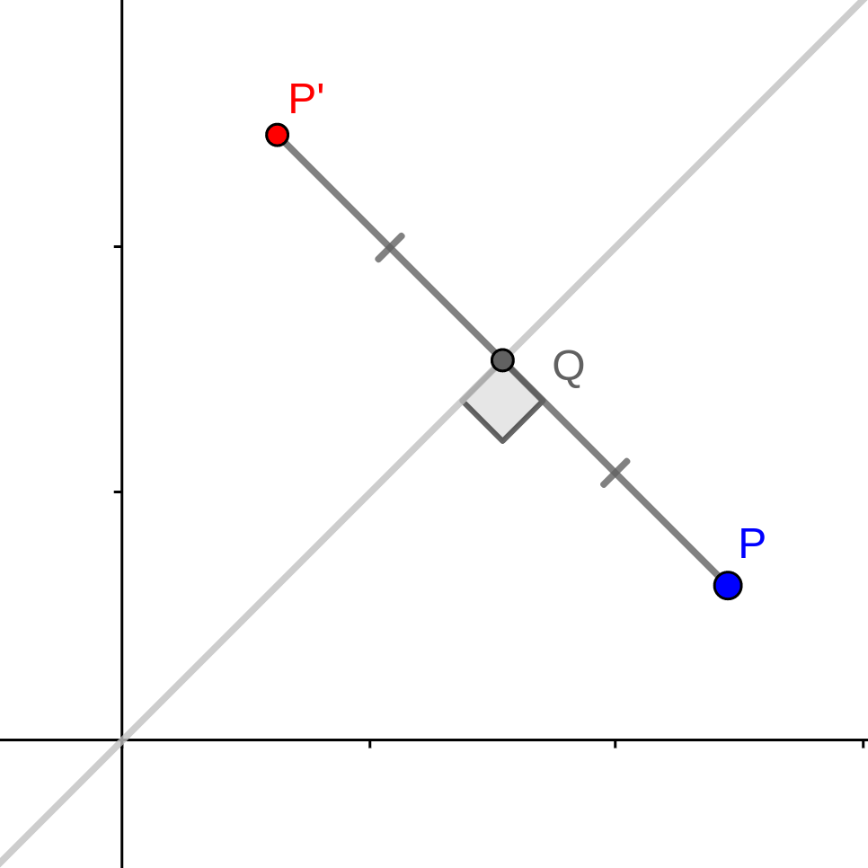
Draw a line segment from $P$ directly left until it intersects the line $y = x$. Draw another line segment from $P'$ directly down until it too intersects the line $y = x$. These two line segments and the line $y = x$ all meet at the same point. Let’s call this point $R$.

Since the line segment $PR$ is horizontal and $P'R$ is vertical, then angle $\angle PRP'$ is a right angle. The other angles $\angle RPP'$ and $\angle RP'P$ are each 45 degrees, so this makes the triangle $\triangle PRP'$ an isosceles triangle.

Now suppose $P$ has the coordinates $(a, b)$. Let’s try to find the coordinates of $P'$.

The triangle $\triangle PRP'$ is an isosceles triangle, so the lengths $\overline{PR}$ and $\overline{P'R}$ are equal. What’s more, $R$ and $P$ have the same $y$-coordinate (we only moved in the $x$ direction to get to $R$) and $R$ and $P'$ have the same $x$-coordinate. We just need to determine how far $R$ is from $P$. To get from $P$ to $P'$, we subtract that distance from the $x$-coordinate and add it to the $y$-coordinate.

Since $P = (a, b)$ is to the lower-right of $y = x$, its $x$-coordinate is larger than the $y$-coordinate, so $a > b$. Since $R$ is on the line $y = x$, its $x$- and $y$-coordinates are equal. But we know $R$ has the same $y$-coordinate as $P$, so $R = (b, b)$. The distance from $P$ to $R$ is just the difference between $a$ and $b$, so $\overline{PR} = a - b$.

Now

\[\begin{align*} P' &= (a - \overline{PR}, b + \overline{PR}) \\ &= (a - (a - b), b + (a - b)) \\ &= (a - a + b, b + a - b) \\ &= (b, a). \end{align*}\]

This argument depended on $P$ being to the lower-right of the line $y = x$. As an exercise, figure out how this argument has to change if $P$ is to the upper-left instead.

Now let’s reflect the graph of a function across the line $y = x$. As always, we sample a bunch of points on the curve, and reflect them each across the line $y = x$. See what happens when we sample more and more points on the graph of $y = x^2$.

%%html
<iframe scrolling="no" title="Reflection-s3" src="https://www.geogebra.org/material/iframe/id/ckvgsvyu/width/598/height/560/border/888888/sfsb/true/smb/false/stb/false/stbh/false/ai/false/asb/false/sri/false/rc/false/ld/false/sdz/false/ctl/false" width="598px" height="560px" style="border:0px;"> </iframe>

We started with a parabola opening upwards. Its reflection is a parabola opening sideways. This has an important implication: the reflection of a function across $y = x$ might not pass the vertical line test!

Keep this in mind while we see how to reflect a function across $y = x$. Points on the graph of an arbitrary function $y = f(x)$ have the form $(x, f(x))$. Their reflections have the form $(f(x), x)$, but this is the same “form” as $(f(y), y)$. Points of that form are just the points on the graph of $x = f(y)$.

Rule: The reflection of a function $y = f(x)$ across the line $y = x$ is the function $x = f(y)$.

This rule tells us that we only need to swap the $x$’s and $y$’s in our function to get its reflection across $y = x$.

Example: Let’s reflect the function $y = x^2$ across the line $y = x$. According to our rule, we just swap the $x$’s and $y$’s. So the reflection is

\[ x = y^2. \]

The problem is solved at this point, but suppose we try to solve for $y$. We get either

\[ y = \sqrt x \]

or

\[ y = -\sqrt x. \]

How do the graphs of $x = y^2$, $y = \sqrt x$, and $y = -\sqrt x$ compare to one another? The graph of $x = y^2$ is a sideways parabola and does not pass the vertical line test. The graph of $y = \sqrt x$ is just the top half of that parabola and therefore does pass the vertical line test. The graph of $y = -\sqrt x$ is the bottom half of the parabola and also passes the vertical line test.

Example: Now let’s reflect the straight line $y = \frac 1 2 x + 1$ across the line $y = x$. Our rule says we just need to swap the $x$’s and $y$’s, so we get

\[ x = \frac 1 2 y + 1. \]

Once again, the problem is solved at this point, but let’s try solving for $y$:

\[ y = 2 x - 2. \]

The reflection of the line $y = \frac 1 2 x + 1$ across the line $y = x$ is the line $y = 2 x - 2$. This is a case of a function whose reflection actually does pass the vertical line test and can be written in the form $y = f(x)$.

Use the interactive graph below to plot functions and their reflections across $y = x$.

%%html
<iframe scrolling="no" title="Reflection-i3" src="https://www.geogebra.org/material/iframe/id/m9xzwneq/width/650/height/548/border/888888/sfsb/true/smb/false/stb/false/stbh/false/ai/false/asb/false/sri/false/rc/false/ld/false/sdz/false/ctl/false" width="650px" height="548px" style="border:0px;"> </iframe>

Reflections combined with function operations¶

We might be asked to reflect a function after performing some function operations. For example, we might be asked to add two functions and the reflect them across the $x$-axis, or reflect the composition of two functions across the $y$-axis. Well, the sum of two functions, for instance, is a function and we know how to reflect functions now, so we ought to be able to do this.

Problem: Reflect $f(x) + g(x)$ across the $x$-axis, where $$ f(x) = x^2 + 1 \text{ and } g(x) = x^3 + 1. $$

Solution: To do this, let’s add $f(x)$ and $g(x)$ and call their sum $h(x)$. So

\[\begin{align*} h(x) &= f(x) + g(x) \\ &= (x^2 + 1) + (x^3 + 1) \\ &= x^3 + x^2 + 2. \end{align*}\]

Now we just need to reflect $h(x)$ across the $x$-axis. Its reflection is $y = -h(x)$, so

\[\begin{align*} y &= -h(x) \\ &= -(x^3 + x^2 + 2) \\ &= -x^3 - x^2 - 2. \end{align*}\]

Problem: Reflect $f(g(x))$ across the $y$-axis, where $$ f(x) = \sin(x) \text{ and } g(x) = x^2. $$

Solution: Like before, let’s compose $f(x)$ and $g(x)$ and call their composite $h(x)$. So

\[\begin{align*} h(x) &= f(g(x)) \\ &= f(x^2) \\ &= \sin(x^2). \end{align*}\]

Now we reflect $h(x)$ across the $y$-axis. The reflection of $h(x)$ is $y = h(-x)$, so

\[\begin{align*} y &= h(-x) \\ &= \sin((-x)^2) \\ &= \sin(x^2). \end{align*}\]

Reflections combined with translations¶

We can apply the same idea above to reflect translations of graphs.

Problem: Translate the function $y = f(x)$ left by three units, then reflect across the $y$-axis, where $y = |2x|$.

Solution: Let’s label by $g(x)$ the translation of $f(x)$ left by three units. Then we just have to reflect $g(x)$ across the $y$-axis. So

\[\begin{align*} g(x) &= f(x+3) \\ &= |2(x+3)| \\ &= |2x + 6|. \end{align*}\]

Its reflection across the $y$-axis is

\[\begin{align*} y &= g(-x) \\ &= |2(-x) + 6| \\ &= |-2x + 6|. \end{align*}\]

Conclusion¶

In this notebook, we saw how to reflect over the $x$-axis, the $y$-axis, the line $y = x$, and combining reflection. We’ve also made a distinction between reflecting a point, reflecting the graph of a function, and reflecting the function itself. Reflections of points and graphs are geometric ideas, manipulating plots; reflections of functions is about manipulating equations, although

The studies of statistics and of the sciences depend heavily on the skills learned in later math courses, especially Calculus courses. A lot of time is spent in Calculus courses analyzing functions and to do this, it is usually helpful to have a clear image in one’s mind of the function being analyzed. Understanding reflections of graphs and functions is one step towards forming such a clear image. For instance, you might already know what the graph of $y = 10^x$ looks like, but using the techniques covered in this notebook, you can also tell what $y = -10^x$, $y = 10^{-x}$, $y = -10^{-x}$, and $x = 10^y$ look like.

Recognizing when a function is “even” or “odd” also has its uses. A typical question in a Calculus class is to find the area underneath a curve and above the $x$-axis. If the curve is given by an even function, then the area to the right of the $y$-axis is the same as the area to the left. That means we can get away with only calculating half the area and then doubling the result. Doubling a number is easier than most things in math, so this can be a time saver.

Exercises¶

Plot the point $(1, 2)$ as well as its reflections across the $x$-axis, the $y$-axis, both axes, and the line $y = x$.
Graph the function $y = x^2 - 2x$. Plot its reflection across the $x$-axis and the $y$-axis. What are the equations of these reflections?
Graph the function $y = e^x$. Plot its reflection across the line $y = x$. Does the reflected function pass the vertical line test? What is the equation of its reflection (in the form $x = f(y)$ and in the form $y = f(x)$)?

from IPython.display import HTML

HTML('''<script>
code_show=true; 
function code_toggle() {
 if (code_show){
 $('div.input').hide();
 } else {
 $('div.input').show();
 }
 code_show = !code_show
} 
$( document ).ready(code_toggle);
</script>
<form action="javascript:code_toggle()"><input type="submit" value="Click here to toggle on/off the raw code."></form>''')

Callysto Curriculum Notebooks

Reflections of Graphs¶

Introduction¶

Reflections across the \(x\)-axis¶

Points¶

Graphs¶

Functions¶

Reflections across the \(y\)-axis¶

Points¶

Graphs¶

Functions¶

Reflections across both axes¶

Even and odd functions¶

Reflections across the line \(y = x\)¶

Points¶

Reflections combined with function operations¶

Reflections combined with translations¶

Conclusion¶

Exercises¶