Inductive Reasoning and Deductive Reasoning¶

There are two forms of reasoning that that are useful when investigating a piece of mathematics.

Inductive reasoning involves looking for patterns in evidence in order to come up with conjectures (i.e. things that are likely to be true). This sort of reasoning will not tell you whether or not something actually is true but it is still very useful for making connections and figuring out what to investigate next.
Deductive reasoning involves starting with what you know and logically figuring out if some conjecture must also be true (and why). While deductive reasoning is stronger than inductive reasoning, it can also be more difficult to use.

In practice, one will often use inductive reasoning to make conjectures and deductive reasoning to verify them. In some cases producing a conjecture will require a mix of inductive and deductive reasoning.

In this notebook we will go over some example problems to help illustrate how one would go about using inductive and deductive reasoning in problem solving while avoiding pitfalls. Being able to apply these skills will make you a more effective problem solver. Being able to distinguish between the two will help you maintain a clear understanding of what you’re doing, why you’re doing it, and avoid mistakes in the process.

A Flawed Application of Inductive Reasoning¶

Consider a circle. Suppose we were to add a certain number of dots to the edge of the circle and then draw chords connecting every pair of dots. The chords would partition the circle into a certain number of regions. Can we find a relationship between the number of dots and the number of regions? For instance, a circle with a two dots along the edge has one chord connecting them and is partitioned into two regions but a circle with three dots along the edge has three chords and is partitioned into four regions.

Here is a simple applet to help visualize the problem. The slider at the bottom controls the number of dots along the edge (from $1$ to $6$). I’ve labeled each region with a number to make them easier to count.

%%html
<iframe scrolling="no" title="cc-20-chords" src="https://www.geogebra.org/material/iframe/id/d4uwgs5k/width/700/height/700/border/888888/sfsb/true/smb/false/stb/false/stbh/false/ai/false/asb/false/sri/false/rc/false/ld/false/sdz/false/ctl/false" width="700px" height="700px" style="border:0px;"> </iframe>

If we look at the number of regions in the first five examples

dots	regions
1	1
2	2
3	4
4	8
5	16

and apply inductive reasoning then we may convince ourselves that the circle with $n$ dots will have $2^{n-1}$ regions.

Is that true? Note: If our inductive reasoning is correct then the sixth case will have $2^{6-1}=32$ regions.

Unfortunately, as it turns out the sixth circle will break down into $31$ regions, not $32$ regions. This is an example where inductive reasoning can lead you astray. Fortunately for us we managed to find a counterexample right away but there are conjectures where the first counterexample took decades to find and required numbers so large that it’s virtually impossible for people to find them by hand. So we should always be very skeptical about the things inductive thinking may lead us to believe.

Some Flawed Applications of Deductive Reasoning¶

Deductive reasoning can also fail us if we are not careful. It is possible to get caught up manipulating equations and not realize there’s an underlying logical problem.

Here are two flawed proofs. Try and find the problem in each one!

A Classic Flawed Proof¶

There are a few variations of this proof (with the same flaw) floating around. Every so often a student rediscovers it and thinks they’ve broken math.

Let $a=b$.

Then it follows that $b^2=ab$.

\[\begin{split} \begin{align*} a^2 - b^2 &= a^2 - b^2\\ a^2 - b^2 &= a^2 - ab \tag{Since $b^2=ab$}\\ (a+b)(a-b) &= (a)(a-b) \tag{Factoring}\\ a+b &= a \tag{Divide by sides by $a-b$}\\ 2a &= a \tag{Since $a=b$}\\ 2 &= 1 \tag{Divide both sides by $a$} \end{align*} \end{split}\]

Hint: The problem involves division.

The problem is introduced when both sides are divided by $a-b$ because $a-b=0$ and division by zero is not allowed (for reasons like this).

A Flawed Proof Involving Radicals¶

This one is somewhat less common but still interesting.

\[\begin{split} \begin{align*} -1 &= i^2 \\ &= (i)(i) \\ &= \sqrt{-1}\sqrt{-1} \\ &= \sqrt{(-1)(-1)} \\ &= \sqrt{1} \\ &= 1 \end{align*} \end{split}\]

So $-1=1$.

Hint: The problem involves distributing roots.

The problem occurs because $\sqrt{ab}=\sqrt{a}\sqrt{b}$ only holds when $a$ and $b$ are both greater than or equal to $0$ (neither $a$ nor $b$ are allowed to be negative).

Some Applications of Inductive Reasoning¶

Sum of the first n odd integers¶

Suppose you need to compute the sum of the first $100$ odd integers. You could do this directly but that likely wouldn’t be very fun or interesting. Let’s instead try applying inductive reasoning to try to come up with a better way to do it.

Before we can start looking for patterns we’ll first need to generate some examples (so that we can use them as evidence later). Let’s do that in Python:

# Create a list of odd integers from 1 to 20 (incrementing by 2 each time).
oddIntegers = range(1,20,2)

# Print a nice heading.
print('|  n | Odd | S(n)|')
print('------------------')

# For each odd integer print the step, the integer, and the sum of all odd integers so far.
step = 0
oddSum = 0
for odd in oddIntegers:
    step = step + 1
    oddSum = oddSum + odd
    print('|{:3d} | {:3d} | {:3d} |'.format(step, odd, oddSum))

|  n | Odd | S(n)|
------------------
|  1 |   1 |   1 |
|  2 |   3 |   4 |
|  3 |   5 |   9 |
|  4 |   7 |  16 |
|  5 |   9 |  25 |
|  6 |  11 |  36 |
|  7 |  13 |  49 |
|  8 |  15 |  64 |
|  9 |  17 |  81 |
| 10 |  19 | 100 |

For brevity we’ll use $S(n)$ to refer to the sum of the first $n$ odd integers.

The code above gives us a list of the first $10$ odd integers as well as $S(n)$ for each one (eg. for $n=3$, the $3$rd odd is $5$ and $S(3) = 1 + 3 + 5 = 9$).

Now look closely at the data and try to see if there is a pattern there. Maybe consider changing the 20 in range(1,20,2) to a larger value to obtain more examples.

Hint: $1+3+5=3^2$.

A good conjecture might be that

\[S(n)=n^2.\]

Here is a slider that tests our conjecture against a larger range of values:

num = widgets.IntSlider(description='n:', min=1)
def oddCompare(num):
    oddIntegers = range(1, num*2, 2)
    oddSum = sum(list(oddIntegers))
    print('S(n): {}'.format(oddSum))
    print('n^2: {}'.format((num*num)))

out = widgets.interactive_output(oddCompare, {'num': num})
widgets.VBox([num, out])

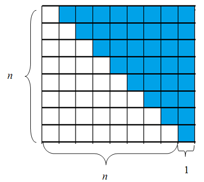
Now that we have a conjecture it is typically very helpful if we’re able to take it further and come up with some guesses about why the conjecture holds. In this case the trick is to realize that we can compute the sum of the first $n$ odd integers by taking the sum of the first $n-1$ odd integers and adding the $n$’th odd. In other words:

\[S(n+1)=S(n) + (n+1)^{\text{th}} \text{ odd integer}.\]

For instance, $S(5) = 1 + 3 + 5 + 7 + 9 = S(4) + 9$.

Then combining this insight with the fact that we can represent square integers as squares yields this visualization:

Odds

https://www.quora.com/What-is-the-sum-of-1+3+5+7+9+11+13+15+17+19+21+23+25+27+29+31+-+95+97+99

Unfortunately as convincing as this visual representation may be, it isn’t strong enough to prove that $S(n)=n^2$ holds for all integers $n$. In order to prove that it holds for all $n$ we require a more advanced proof technique that we don’t currently have access to. So we must grit our teeth and accept the fact that as far as we know there could exist some integer out there for which this fails. Despite this some people will accept the visual argument as a proof because it provides the key intuition necessary to develop a proof.

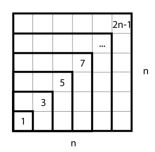
Triangular numbers¶

There is famous story about the mathematician Carl Friedrich Gauss who as a child in primary school was tasked with computing the sum of the first 100 integers as a way to keep him busy. As the story goes, Gauss quickly realized a pattern and wrote down the answer of 5050 within a few seconds.

For brevity we’ll use $T(n)$ to refer to the sum of the first $n$ integers.

The trick to seeing the pattern in this problem isn’t as straightforward as the last one. As before we’ll need to generate some examples to analyze first.

# Create a list of the first 10 integers.
integers = range(1,11)

# Print a nice heading.
print('|  n  | T(n)|')
print('-------------')

# For each integer print the integer and the sum of all integer so far.
tSum = 0
for num in integers:
    tSum = tSum + num
    print('| {:3d} | {:3d} |'.format(num, tSum))

|  n  | T(n)|
-------------
|   1 |   1 |
|   2 |   3 |
|   3 |   6 |
|   4 |  10 |
|   5 |  15 |
|   6 |  21 |
|   7 |  28 |
|   8 |  36 |
|   9 |  45 |
|  10 |  55 |

Unfortunately this didn’t turn out to be very insightful.

Another approach we can take is to try to represent the sum differently. Taking a cue from the previous section we’ll draw the sum visually:

Triangle Number

https://www.chegg.com/homework-help/use-ideas-behind-drawings-b-find-solution-gauss-s-problem-ex-chapter-1.1-problem-2a-solution-9780321987297-exc

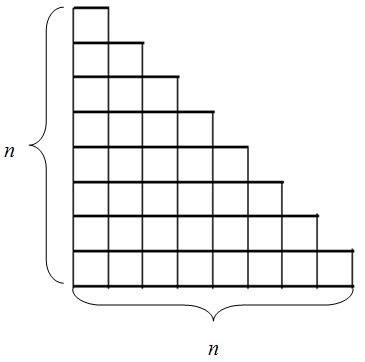
It is because of this representation that the sum of the first $n$ integers is often referred to as a $n$’th triangle number. The value of our sum is represented by the ‘area’ of its triangular representation. Now, while it may not be easy to compute the area of such a triangle it is easy to compute the area of a rectangle and we can produce one by setting two triangles face to face:

Triangle Number Sum

https://www.chegg.com/homework-help/use-ideas-behind-drawings-b-find-solution-gauss-s-problem-ex-chapter-1.1-problem-2a-solution-9780321987297-exc

This representation suggests a good conjecture for computing the $n$’th triangle number: $$T(n)=\frac{(n)(n+1)}{2}.$$

Unfortunately we once again lack the advanced proof technique we need to prove (using deductive thinking) that this is true for all integers $n$. So like before we’ve managed to obtain a really good conjecture through inductive thinking but are not able to confirm with certainty whether or not it’s true. Like the previous example, some people may accept this visual argument as a proof.

One Weird Trick¶

From time to time neat computational tricks like this will go viral on social media. Unfortunately the people presenting them will typically only show a few flashy examples and leave the readers feeling completely mystified about why the trick works (or worse, feeling betrayed when it fails).

One Weird Trick

https://brightside.me/article/nine-simple-math-tricks-youll-wish-you-had-always-known-92805/

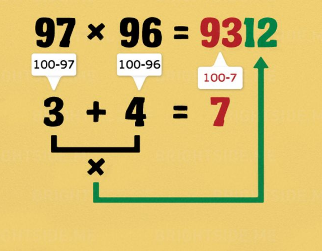
Before we start lets first rephrase what the picture is saying:

To compute $(97)(96)$:

For each of our values, compute their difference from $100$:

$3=100-97$
$4=100-96$

Multiply the differences to compute the first two digits of the result:

$12=(3)(4)$

Add the differences and subtract the result from $100$ to compute the remaining digits of the result:

$93=100-(3+4)$

Glue the two results together to get the final result:

$(97)(96)=9312$

It looks like step 3 could be simplified a bit to $93 = 97 - 4$ or $93 = 96 - 3$

In general it looks like the algorithm may be something like this:

To compute $(a)(b)$:

For each of our values, compute their difference from $100$:

$a'=100-a$
$b'=100-b$

Multiply the differences to compute the last two digits of the result:

$D=(a')(b')$

Add the differences and subtract the result from $100$ to compute the remaining digits of the result:

$C=a-b'$

Glue the two results together to get the final result:

$(a)(b)=C\text{ appended with }D$

Next lets have the computer generate some more examples for us so that we can get a better sense of the problem through inductive reasoning. The two sliders below let us choose some inputs and present the result created by the algorithm as well as the actual result with a message saying Success! if the algorithm gave the correct answer and Fail! if it gave the incorrect answer.

a = widgets.IntSlider(description='a:', min=85, max=115, value=100)
b = widgets.IntSlider(description='b:', min=85, max=115, value=100)

def multiply(a,b):
    aDiff = 100-a
    bDiff = 100-b
    
    firstTwo = aDiff*bDiff
    lastTwo = a - bDiff
    
    result = str(lastTwo).lstrip('0') + str(firstTwo).zfill(2)
    print('Result: {}'.format(result))
    print('Actual product: {}'.format((a*b)))
    if (result == str(a*b)):
        print('Success!')
    else:
        print('Fail!')

out = widgets.interactive_output(multiply, {'a': a, 'b':b})
widgets.VBox([a,b, out])

Playing around with the sliders it seems that the algorithm fails in two cases:

Where the first digits in the result are greater than $100$.
- for instance, for $(101)(99)$ it gives 100-1 instead of 9999
Where the first digits in the result are negative.
- For instance, for $(110)(110)$ it gives 120120 instead of 12100

Can you see a pattern in the way the numbers fail, maybe a way to fix it?

It seems like both instances can be fixed by carrying values. Perhaps, instead of gluing values together like strings we’re actually supposed to be multiplying the last digits by $100$ and adding the first digits! For instance, instead of saying $$9312 = 93\text{ appended with }12$$ we would say $$9312=(93)(100)+12.$$

Lets update the algorithm with this change:

To compute $(a)(b)$:

For each of our values, compute their difference from $100$:

$a'=100-a$
$b'=100-b$

Multiply the differences to compute the first two digits of the result:

$D=(a')(b')$

Add the differences and subtract the result from $100$ to compute the remaining digits of the result:

$C=a - b'$

Combine the two results together to get the final result:

$(a)(b)=(C)(100) + D$

In other words: $$ab = [a-(100-b)](100) + (100-b)(100-a).$$

Next let’s create a new version of the sliders:

a = widgets.IntSlider(description='a:', min=85, max=115, value=100)
b = widgets.IntSlider(description='b:', min=85, max=115, value=100)

def multiply(a,b):
    aDiff = 100-a
    bDiff = 100-b
    
    firstTwo = aDiff*bDiff
    lastTwo = 100 - (aDiff + bDiff)
 
    result = lastTwo*100 + firstTwo
    print('Result: {}'.format(result))
    print('Actual product: {}'.format((a*b)))
    if (result == a*b):
        print('Success!')
    else:
        print('Fail!')

out = widgets.interactive_output(multiply, {'a': a, 'b':b})
widgets.VBox([a,b, out])

For the two failing examples mentioned above we now get:

For $(101)(99)$ we get 9999 which is correct!
For $(110)(110)$ we get 12100 which is correct!

Now that we have a conjecture let’s getting a better sense of why it works. One thing we can do is to take our equation from above:

\[\begin{split} \begin{align} ab &= [a-(100-b)](100) + (100-b)(100-a) \\ &= (a)(100) - (100-b)(100) + (100-b)(100-a) \end{align} \end{split}\]

We can visualize this:

%%html
<iframe scrolling="no" title="cc-20-weird-trick" src="https://www.geogebra.org/material/iframe/id/cb88dnrd/width/732/height/415/border/888888/sfsb/true/smb/false/stb/false/stbh/false/ai/false/asb/false/sri/false/rc/false/ld/false/sdz/false/ctl/false" width="732px" height="415px" style="border:0px;"> </iframe>

Note: This visualization assumes that $a$ and $b$ are between $0$ and $100$ (though in our conjecture we also allow them be greater than $100$).

In general these sorts of techniques where one performs a computation by manipulating the digits of a value is called an ‘algorism’ (not to be confused with algorithm). They’re not really used very much these days (except for fast mental math gimmicks).

This particular algorism has a lot of generalizations for dealing with larger numbers but the reasoning behind them gets quite convoluted and in the end the most important part isn’t proving that a algorism works for all numbers but that it works for all the numbers for which a mental computation is fast. In this case we can be satisfied by saying that this algorism works for numbers between $91$ and $109$ since those values are the easiest to use in practice.

Some Applications of Deductive Reasoning¶

Fractions¶

Fractions can be difficult to manipulate. Perhaps we can use deductive reasoning to come up with some easier ways to manipulate them.

First some observations:

Any integer, like $3$, can be written in fraction form:

\[ 3=\frac{3}{1}. \]

Any integer except $0$, like $3$, can be put into a fraction to get $1$:

\[ 1=\frac{3}{3}. \]

In order to multiply two fractions, such as $\frac{2}{3}$ and $\frac{5}{7}$, just multiply the numerators and denominators:

\[ \left( \frac{2}{3}\right) \left( \frac{5}{7} \right) = \frac{(2)(5)}{(3)(7)} = \frac{10}{21}. \]

The first thing to note is that observation (3) gives us a way to factor any fraction:

\[ \frac{2}{3} = \left( \frac{2}{1}\right) \left( \frac{1}{3} \right). \]

Reducing a fraction, such as $\frac{10}{15}$ to $\frac{2}{3}$, can be achieved by applying observations (2) and (3) in reverse:

\[ \frac{10}{15}=\frac{(2)(5)}{(3)(5)}=\left(\frac{2}{3}\right)\left(\frac{5}{5}\right)=\left(\frac{2}{3}\right)(1)=\frac{2}{3} \]

The usual process of cancelling a denominator, like $(3) \left(\frac{2}{3}\right)=2$ follows from these observations as well:

\[ (3) \left(\frac{2}{3}\right) = \left(\frac{3}{1}\right) \left(\frac{2}{1}\right)\left(\frac{1}{3}\right) = \left(\frac{3}{3}\right) \left(\frac{2}{1}\right) = (1)(2) = 2 \]

Let’s use these observations to manipulate some more complicated fractions.

\[\begin{split} \begin{align*} \frac{2}{\frac{1}{5}} & = \left( \frac{2}{\frac{1}{5}}\right) (1) \tag{Multiply by $1$}\\ & = \left( \frac{2}{\frac{1}{5}}\right) \left(\frac{5}{5} \right) \tag{By observation 2}\\ & = \frac{(2)(5)}{\left( \frac{1}{5}\right) (5)} \tag{By observation 3}\\ & = \frac{(2)(5)}{1} \tag{By cancelling}\\ & = (2)(5) \tag{By observation 1}\\ & = 10 \end{align*} \end{split}\]

Another more complicated example:

\[\begin{split} \begin{align*} \frac{\frac{2}{3}}{\frac{7}{5}} & = \left( \frac{\frac{2}{3}}{\frac{7}{5}} \right) (1)(1) \tag{Multiply by $1$}\\ & = \left( \frac{\frac{2}{3}}{\frac{7}{5}} \right) \left(\frac{3}{3} \right)\left(\frac{5}{5} \right) \tag{By observation 2}\\ & = \frac{\left( \frac{2}{3} \right) (3)(5)}{\left(\frac{7}{5} \right) (3)(5)} \tag{By observation 3}\\ & = \frac{(2)(5)}{(7)(3)} \tag{By cancelling}\\ & = \frac{10}{21} \end{align*} \end{split}\]

We can manipulate even the most complicated fractions by cleverly multiplying by 1 in this way.

Distributive Property¶

The distributive property is extremely useful in simplifying expressions and performing computations. In fact, every multiplication algorithm you encounter will at some level boil down to some clever application of the distributive property. Simply put the distributive property tells us how addition and multiplication interact:

\[ (a+b)c = ac + bc. \]

Since multiplication is commutative this statement is equivalent:

\[ a(c+d) = ac + ad. \]

The FOIL mnemonic is just a special case of the distributive property:

\[ (a+b)(c+d) = (a+b)c + (a+b)d = ac + bc + ad + bd. \]

It is important to remember that the distributive property can be read two ways. In one sense it tells us how to distribute multiplication across addition but in another sense it tells us how to undo that distribution.

For an example, suppose you have something like

\[ 6x + 10xy. \]

If we notice that both $6x$ and $10xy$ have $2x$ as a factor, since $6x=2x(3)$ and $10xy=2x(5y)$, then we can rewrite that as

\[ 6x + 10xy = 2x(3 + 5y). \]

This technique is an extremely useful application of deductive reasoning. Do not underestimate it.

Mentally Computing Simple Percentages¶

There are many occasions where one might be asked to compute a percentage of some value on the spot (eg. tipping at a restaurant). Fortunately there’s a trick to doing it quickly.

First notice that computing $10\%$ is as easy as moving the decimal point one digit to the left (eg. $10\%$ of $25.3$ is $2.53$). Similarly, $1\%$ can be computed by moving the decimal point two digits to the left.

From there on it’s just a matter of adding, subtracting, and/or multiplying these percentages to get to the desired percentage. For instance, $18\%$ can be computed by first computing $10\%$, doubling the value to get $20\%$, moving the decimal over one more time to get $2\%$ and then subtracting the $2\%$ value from the $20\%$ value. It’s easier than it sounds.

This is an application of deductive reasoning because we reached all of the assertions here logically, not by looking at any patterns and conjecturing.

Callysto Curriculum Notebooks