Fibonacci Numbers¶

The Fibonacci sequence is the set of numbers that starts out like this:

\[0,1,1,2,3,5,8,13,\ldots.\]

It’s easy to recognize the pattern here. Each number is the sum of the previous two numbers in the sequence. Except, of course, the first two number, 0 and 1, which we put in there to get things started.

This sequence, or pattern of numbers, goes on forever.

These numbers are most commonly known as the Fibonacci numbers, after the Italian mathematician L. Fibonacci (c. 1200 C.E.). However, these numbers were actually first described hundreds of years before, by Indian mathematicians. The first such mathematician for whom we have written records was Virahanka (c. 700 C.E.).

It is difficult to overcome the usage of a name adopted hundreds of years ago, and so in what follows we will refer to the Virahanka-Fibonacci numbers as the “Fibonacci numbers.”

Exercise 1: Check out the following article about the “so-called Fibonacci” numbers in ancient India: https://www.sciencedirect.com/science/article/pii/0315086085900217

For an excellent exposition about the motivation, poetry, and linguistics of these early mathematicians, and to learn about some fascinating properties of these numbers, check out the following video:

from IPython.display import YouTubeVideo
YouTubeVideo('LP253wHIoO8', start=2633)

It’s convenient to label these numbers, so we write $F_0 = 0$, $F_1 = 1$ $F_2 = 2$ and so on. The list of numbers is thus defined recursively by the formula $ \qquad$$ F_n = F_{n-1} + F_{n-2}.$

We can check the few numbers in the Fibonacci sequence are obtained by that formula, by computing:

\[\begin{split}\begin{eqnarray*} F_{2} &=&F_{1}+F_{0}=1+0=1 \\ F_{3} &=&F_{2}+F_{1}=1+1=2 \\ F_{4} &=&F_{3}+F_{2}=2+1=3 \\ F_{5} &=&F_{4}+F_{3}=3+2=5 \\ F_{6} &=&F_{5}+F_{4}=5+3=8 \\ F_{7} &=&F_{6}+F_{5}=8+5=13 \\ &&\vdots \end{eqnarray*} \end{split}\]

Here is a list of the first 40 Fibonacci numbers:

\[\begin{split} \begin{array}{rrrrrrrrrrrrrrr} 0 & & 1 & & 1 & & 2 & & 3 & & 5 & & 8 & & 13 \\ & & & & & & & & & & & & & & \\ 21 & & 34 & & 55 & & 89 & & 144 & & 233 & & 377 & & 610 \\ & & & & & & & & & & & & & & \\ 987 & & 1597 & & 2584 & & 4181 & & 6765 & & 10946 & & 17711 & & 28657 \\ & & & & & & & & & & & & & & \\ 46368 & & 75025 & & 121393 & & 196418 & & 317811 & & 614229 & & 832040 & & 1346269 \\ & & & & & & & & & & & & & & \\ 2178309 & & 3524578 & & 5702887 & & 9227465 & & 14930352 & & 24157817 & & 39088169 & & 63245986% \end{array}\end{split}\]

Exercise 2: Write a code that computes the first N Fibonacci numbers, saves them into an array, and displays them on the screen.

WAIT – before you read the next cell, try to do Exercise 2!

N = 20   # Set the size of the list we will compute

F=[0,1]  # The first two numbers in the list
for i in range(2, N):
    F.append(F[i-1]+F[i-2])  # append the next item on the list

print('First',N,'Fibonacci numbers:',F)

For fun, we can make a little widget to control how many numbers to print out.

from ipywidgets import interact

def printFib(N=10):
    F=[0,1]  # The first two numbers in the list
    for i in range(2, N):
        F.append(F[i-1]+F[i-2])  # append the next item on the list
    print(F)
    
interact(printFib, N=(10,100,10));

By moving the slider above, print out the first 100 Fibonacci numbers

As we can see, this sequence grows pretty fast. The Fibonacci numbers seem to have one more digit after about every five terms in the sequence.

How fast does it grow?¶

One of the ways to study the growth of a sequence is to look at ratios between consecutive terms. We look at ratios of pairs of numbers in the Fibonacci sequence.

The first few values are

(23)¶\[\begin{eqnarray} F_2/F_1 &=& 1 \\ F_3/F_2 &=& 2/1 = 2 \\ F_4/F_3 &=& 3/2 = 1.5 \\ F_5/F_4 &=& 5/3 = 1.666... \\ F_6/F_5 &=& 8/5 = 1.6 \\ F_7/F_6 &=& 13/8 = 1.625 \end{eqnarray}\]

So the ratios are levelling out somewhere around 1.6. We observe that $1.6^5 \approx 10$, which is why after every five terms in the Fibonacci sequence, we get another digit. This tells us we have roughly exponential growth, where $F_n$ grows about as quickly as the exponential function $(1.6)^n$.

We can check this computation in Python. We use $ ** $ to take a power, as in the following cell.

(1.6)**5

The Golden Ratio¶

We can print out a bunch of these ratios, and plot them, just to see that they do. The easiest way to do this is with a bit of Python code. Perhaps you can try this yourself.

Exercise 3 Write some code that computes the first N ratios $F_{n+1}/F_n$, save them it into an array, and displays them on the screen.

WAIT! Don’t read any further until you try the exercises.

%matplotlib inline
from matplotlib.pyplot import * 

N = 20
F = [0,1]
R = []
for i in range(2, N):
    F.append(F[i-1]+F[i-2])  # append the next item on the list
    R.append(F[i]/F[i-1])


figure(figsize=(10,6));
plot(R,'o')
title('The first '+str(N-2)+' Ratios $F_{n+1}/F_n$')
xlabel('$n$')
ylabel('$Ratio$');

print('The first', N-2, 'ratios are:',R)

We see the numbers are levelling out at the value 1.6108034… This number may be familiar to you. It is called the Golden Ratio.

We can compute the exact value by observing the ratios satisfy a nice algebraic equation: $ \frac{F_{n+2}}{F_{n+1}}=\frac{F_{n+1}+F_{n}}{F_{n+1}}=1+\frac{F_{n}}{F_{n+1}}=1+\frac{1}{\frac{F_{n+1}}{F_{n}}}, $

or more simply

$\frac{F_{n+2}}{F_{n+1}}=1+\frac{1}{\frac{F_{n+1}}{F_{n}}}.$

As $n$ gets larger and larger, the ratios $F_{n+2}/F_{n+1}$ and $F_{n+1}/F_{n}$ tend toward a final value, say $x$. This value must then solve the equation $x=1+\frac{1}{x}.$

We rewrite this as a quadratic equation $x^2=x+1$ which we solve from the quadratic formula $ x= \frac{1 \pm \sqrt{1+4}}{2} = \frac{1 \pm \sqrt{5}}{2}.$ It is the positive solution $x= \frac{1 + \sqrt{5}}{2} = 1.6108034$… which is called the Golden Ratio.

The Golden ratio comes up in art, geometry, and Greek mythology as a perfect ratio that is pleasing to the eye (and to the gods).

For instance, the rectangle shown below is said to have the dimensions of the Golden ratio, because the big rectangle has the same shape as the smaller rectangle inside. Mathematically, we have the ratios of lengths $ \frac{a+b}{a} = \frac{a}{b}.$

Golden ratio rectangle

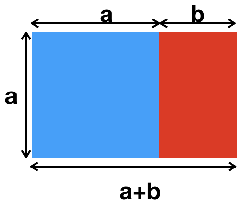
Writing $x = \frac{a}{b}$, the above equation simplifies to $ 1 + \frac{1}{x} = x,$ which is the same quadratic equation we saw for the limit of ratios of Fibonacci numbers.

For more information about the Golden ratio see https://en.wikipedia.org/wiki/Golden_ratio

A Formula for the Fibonacci Sequence $F_n$¶

Let’s give the Golden ratio a special name. In honour of the ancient Greeks who used it so much, we call it `phi:’ $ \varphi = \frac{1 + \sqrt{5}}{2}. $ We'll call the other quadratic root 'psi:' $ \psi = \frac{1 - \sqrt{5}}{2}. $ This number$\psi$ is called the conjugate of $\varphi$ because it looks the same, except for the negative sign in front of the $\sqrt{5}$.

Here’s something amazing. It turns out that we have a remarkable formula for the Fibonnaci numbers, in terms of these two Greek numbers. The formula says $F_n = \frac{\varphi^n - \psi^n}{\sqrt{5}}.$

Wow!¶

Seems amazing. And it is handy because now we can compute, say, the thousandth term in the sequence, $F_{1000}$ directly, without having to compute all the other terms that come before.

But, whenever someone gives you a formula, you should check it!

Exercise 4: Write a piece of code to show that the formula above, with $\varphi,\psi$ does produce, say, the first 20 Fibonnaci numbers.

WAIT! Don’t go on until you try writing a program yourself, to compute the Fibonacci numbers using only powers of $\varphi, \psi$.

## SOLUTION (don't peak!)

from numpy import *  ## We need this to define square roots
phi = (1 + sqrt(5))/2
psi = (1 - sqrt(5))/2
for n in range(20):
    print( (phi**n - psi**n)/sqrt(5) ) 

Looking at that computer output, it does seem to give Fibonacci numbers, with a bit of numerical error.

Checking the Math¶

Doing math, though, we like exact answers and we want to know why. So WHY does this formula $(\phi^n - \psi^n)/\sqrt{5}$ give Fibonacci numbers?

Well, we can check, step by step.

For $n=0$, the formula gives $\frac{\varphi^0 - \psi^0}{\sqrt{5}} = \frac{1-1}{\sqrt{5}} = 0,$ which is $F[0]$, the first Fibonacci number.

For $n=1$, the formula gives $\frac{\varphi^1 - \psi^1}{\sqrt{5}} = \frac{\frac{1 + \sqrt{5}}{2} - \frac{1 -\sqrt{5}}{2} }{\sqrt{5}} = \frac{\sqrt{5}}{\sqrt{5}} = 1,$ which is F[1], the next Fibonacci number.

For $n=2$, it looks harder because we get the squares $\varphi^2, \psi^2$ in the formula. But then remember that both $\varphi$ and $\psi$ solve the quadratic $x^2 = x+1$, so we know $\varphi^2 = \phi +1$ and $\psi^2 = \psi +1$. So we can write $$\frac{\phi^2 - \psi^2}{\sqrt{5}} = \frac{\phi + 1 - \psi -1}{\sqrt{5}} = \frac{\phi - \psi }{\sqrt{5}} = 1,$ since we already calculated this in the $n=1$ step. So this really is F[2]=1.

For $n=3,4,5,\ldots$ again it might seem like it will be hard because of the higher powers. But multiplying the formulas $\varphi^2 = \varphi +1$ and $\psi^2 = \psi +1$ by powers of $\phi$ and $\psi$, we get

\[\begin{split}\begin{eqnarray*} \varphi^2 &=& \varphi +1,\quad \varphi^3 = \varphi^2+\varphi ,\quad \varphi^4=\varphi^3+\varphi^2,\qquad \dots \qquad % \varphi^{n+2}=\varphi^{n+1}+{\varphi}^n,\quad \text{and} \\ \psi^2 &=&\psi +1,\quad \psi^3=\psi^2+\psi ,\quad \psi^4=\psi^3+\psi^2,\qquad \dots \qquad \psi^{n+2}=\psi^{n+1}+\psi^n. \end{eqnarray*}\end{split}\]

So, assuming we know the generating formula already for $n$ and $n+1$ we can write the next term as $$\frac{\varphi^{n+2} - \psi^{n+2}}{\sqrt{5}} = \frac{\varphi^{n+1} +\varphi^n - \psi^{n+1} - \psi^n}{\sqrt{5}} = \frac{\varphi^{n+1} - \psi^{n+1}}{\sqrt{5}} + \frac{\varphi^{n} - \psi^{n}}{\sqrt{5}} = F[n+1] + F[n] = F[n+2].$$

So we do get $\frac{\varphi^{n+2} - \psi^{n+2}}{\sqrt{5}} = F[n+2]$, and the formula holds for all numbers n.

This method of verifying the formula for all n, based on previous values of n, is an example of mathematical induction.

Why did this work?¶

Well, from the Golden ratio, we have the formula $\varphi^2 = \varphi + 1$, which then gives the formula $\varphi^{n+2} = \varphi^{n+1} + \varphi^n$. This looks a lot like the Fibonacci formula $F[n+2] = F[n+1] + F[n].$ Same powers of $ \psi$.

If we take ANY linear combination of powers of $\varphi, \psi$, such as $f(n) = 3\varphi^n + 4\psi^n,$ we will get a sequence that behaves like the Fibonacci sequence, with $f(n+2) = f(n+1) + f(n)$. To get the ‘right’ Fibonacci sequence, we just have to replace the 3 and 4 with the right coefficients.

From sequences to functions¶

Wouldn’t it be fun to extend Fibonacci numbers to a function, defined for all numbers $x$?

The problems is the function $F[x] = \frac{\varphi^x - \psi^x}{\sqrt{5}}$ is not defined for values of $x$ other than integers.

The issue is the term $\psi^{x}=\left( \frac{1-\sqrt{5}}{2}\right) ^{x}$, which is the power of a negative number. We don’t really know how to define that. For instance, what is the square root of a negative number?

To overcome this technical difficulty, we write

\[\psi ^{x}=\left( -\left( -\psi \right) \right) ^{x}=\left( -\left( \frac{% \sqrt{5}-1}{2}\right) \right) ^{x}=\left( -1\right) ^{x}\left( \frac{\sqrt{5}% -1}{2}\right) ^{x}. \]

Now the factor $\left( \frac{\sqrt{5}-1}{2} \right) ^{x}$ make sense since the number inside the brackets is positive. We have localized the problem into the powers of $-1$ for the term $\left( -1\right) ^{x}$. We would like to replace this term by a continuous function $m(x)$ such that it takes the values $\pm1$ on the integers. That is,

\[m(n) =1\quad \text{if }n\text{ is even }\quad\text{and}\quad m(n) =-1\quad \text{if }n\text{ is odd.} \]

The cosine function works. That is

\[m\left( x\right) =\cos \left( \pi x\right) \qquad \text{does the job.} \]

That is: $\cos \left( n\pi \right) =1\quad \text{if }n\text{ is even}\quad\text{ and}\quad % \cos \left( n\pi \right) =-1\quad \text{if }n\text{ is odd.}$

Why this is a good choice would lead us to complex numbers and more!

Hence, we obtain the following closed formula for our function $F[x]:$

\[\begin{split}\begin{eqnarray*} F[x] &=&\frac{{\varphi }^{x}-\left( -1\right) ^{x}\left( -\psi \right) ^{x}}{{\varphi -\psi }}=\frac{1}{\sqrt{5}}\left( {\varphi }% ^{x}-\left( -1\right) ^{x}\left( -\psi \right) ^{x}\right) \\ &=&\frac{1}{\sqrt{5}}\left( \left( \frac{1+\sqrt{5}}{2}\right) ^{x}-\cos \left( \pi x\right) \left( \frac{\sqrt{5}-1}{2}\right) ^{x}\right) . \end{eqnarray*}\end{split}\]

Let’s plot this function, and the Fibonacci sequence.

A plot of the continuous Fibonacci function¶

%matplotlib inline
from numpy import *
from matplotlib.pyplot import *

phi=(1+5**(1/2))/2
psi=(5**(1/2)-1)/2

x = arange(0,10)
y = (pow(phi,x) - cos(pi*x)*pow(psi,x))/sqrt(5)
xx = linspace(0,10)
yy = (pow(phi,xx) - cos(pi*xx)*pow(psi,xx))/sqrt(5)

figure(figsize=(10,6));
plot(x,y,'o',xx,yy);
title('The continuous Fibonacci function')
xlabel('$x$')
ylabel('$Fib(x)$');

A plot with negative values¶

Well, with this general definition, we can even include negative numbers for $x$ in the function.

Let’s plot this too.

%matplotlib inline
from numpy import *
from matplotlib.pyplot import *

phi=(1+5**(1/2))/2
psi=(5**(1/2)-1)/2

x = arange(-10,10)
y = (pow(phi,x) - cos(pi*x)*pow(psi,x))/sqrt(5)
xx = linspace(-10,10,200)
yy = (pow(phi,xx) - cos(pi*xx)*pow(psi,xx))/sqrt(5)


figure(figsize=(10,6));
plot(x,y,'o',xx,yy);
title('The Fibonacci function, extended to negative values')
xlabel('$x$')
ylabel('$Fib(x)$');

So we see we can even get negative Fibonacci numbers!

The Golden Ratio and Continued Fractions¶

We have found that the Golden ratio ${\varphi =}\frac{{1+}\sqrt{5}}{2}$ satisfies the identity

\[ {\varphi =1+}\frac{1}{{\varphi }}. \]

Substituting for ${\varphi }$ on the denominator in the right, we obtain

\[ {\varphi =1+}\frac{1}{{1+}\frac{1}{{\varphi }}}. \]

Substituting again for ${\varphi }$ on the denominator in the right, we obtain

\[ {\varphi =1+}\frac{1}{{1+}\dfrac{1}{{1+}\frac{1}{{\varphi }}}}. \]

Repeating this again,

\[ {\varphi =1+}\frac{1}{{1+}\dfrac{1}{{1+}\dfrac{1}{{1+}\frac{1}{{\varphi }}}}}% .\]

And again,

\[ {\varphi =1+}\frac{1}{{1+}\dfrac{1}{{1+}\dfrac{1}{{1+}\dfrac{1}{{1+}\frac{1}{% {\varphi }}}}}}. \]

And again,

\[ {\varphi =1+}\frac{1}{{1+}\dfrac{1}{{1+}\dfrac{1}{{1+}\dfrac{1}{{1+}\dfrac{1% }{{1+}\frac{1}{{\varphi }}}}}}}. \]

We see that this process can be $\textit{continued indefinitely}$. This results in an $\textit{infinite expansion of a fraction}$. These type of expressions are known as $\textbf{continued fractions}$:

\[ {\varphi =1+}\frac{1}{{1+}\dfrac{1}{{1+}\dfrac{1}{{1+}\dfrac{1}{{1+}\dfrac{1% }{{1+}\dfrac{1}{{1+}\dfrac{1}{1+\dfrac{1}{{\vdots }}}}}}}}}. \]

We can approximate continued fractions with the finite fractions obtained by stopping the development at some point. In our case, we obtain the approximates

\[ 1,~1+1,~1+\frac{1}{1+1},~1+\frac{1}{1+\dfrac{1}{1+1}},~1+\frac{1}{1+\dfrac{1% }{1+\dfrac{1}{1+1}}},~1+\frac{1}{1+\dfrac{1}{1+\dfrac{1}{1+\dfrac{1}{1+1}}}}% ,\dots \]

Explicitly, these approximates are

\[ 1,~2,~\frac{3}{2},~\frac{5}{3},~\frac{8}{5},~\frac{13}{8},\dots \]

This looks like it is just the sequence of ratios $F_{n+1}/F_n$ we saw above! How can we prove this is the case for all $n$?

We know that the sequence $R_{n} = F_{n+1}/F_n$ satisfies the recursive relation.

\[ R_{n}=\frac{F_{n+1}}{F_{n}}=1+\frac{F_{n-1}}{F_{n}}=1+\frac{1}{R_{n-1}}% ,\qquad \text{with}\qquad R_{1}=1. \]

Then, we can generate all the terms in the sequence $R_{n}$ by staring with $% R_{1}=1$, and then using the relation $R_{n+1}=1+\frac{1}{R_{n}}:$

\[\begin{split} \begin{eqnarray*} R_{1} &=&1 \\ R_{2} &=&1+\frac{1}{R_{1}}=1+\frac{1}{1}=2 \\ R_{3} &=&1+\frac{1}{R_{2}}=1+\frac{1}{1+R_{1}}=1+\frac{1}{1+1} \\ R_{4} &=&1+\frac{1}{R_{3}}=1+\frac{1}{1+\frac{1}{1+1}} \\ R_{5} &=&1+\frac{1}{R_{4}}=1+\frac{1}{1+\frac{1}{1+\frac{1}{1+1}}} \\ &&\vdots \end{eqnarray*} \end{split}\]

This confirms that both the sequence of rations $R_{n}$ and the sequence of approximations to the continuous fraction of ${\varphi }$ are the same sequence. $\square $

In general, continued fractions are expressions of the form

\[ a_{0}+\frac{1}{a_{1}+\dfrac{1}{a_{2}+\dfrac{1}{a_{3}+\dots }}} \]

where $a_{0}$ is an integer and $a_{1},a_{2},a_{3},\dots $ are positive integers. These type of fractions are abbreviated by the notation

\[ \left[ a_{0};a_{1},a_{2},a_{3},\dots \right] =a_{0}+\frac{1}{a_{1}+\dfrac{1}{% a_{2}+\dfrac{1}{a_{3}+\dots }}}. \]

For example

\[\begin{split} \begin{eqnarray*} \left[ 1;1,1,2\right] &=&1+\frac{1}{1+\dfrac{1}{1+\dfrac{1}{1+1}}}=\frac{8}{% 5} \\ && \\ \left[ 1;1,1,1,1,\dots \right] &=&{1+}\frac{1}{{1+}\dfrac{1}{{1+}\dfrac{1}{% {1+}\dfrac{1}{{1+}\dfrac{1}{{1+}\dfrac{1}{{1+}\dfrac{1}{1+\dfrac{1}{{\vdots }% }}}}}}}}={\varphi } \end{eqnarray*} \end{split}\]

For more information of continued fractions, see https://en.wikipedia.org/wiki/Continued_fraction

Conclusion¶

What have we learned?¶

a sequence is an ordered list of numbers, which may go on forever.
the Fibonacci sequence 0,1,1,2,3,5,8,13,… is a famous list of numbers, well-studied since antiquity.
each number in this sequence is the sum of the two coming before it in the sequence.
the sequence grows fast, increasing by a factor of about 10 for every five terms.
the ratio of pairs of Fibonacci numbers converges to the Golden ratio, known since the ancient Greeks as the number $\varphi = \frac{1 + \sqrt{5}}{2} \approx 1.6108.$
the Fibonacci numbers can be computed directly as the difference of powers of $\varphi$ and its conjugate, $\psi = \frac{1 - \sqrt{5}}{2}.$ This is sometimes faster than computing the whole list of Fibonnaci numbers.
this formula with powers of $\varphi, \psi$ is verified using induction.
The Fibonacci numbers can be extended to a continuous function $Fib(x)$, defined for all real numbers $x$ (including negatives). It oscillates (wiggles) on the negative x-axis.
The Golden Ratio can also be expressed a continued fraction, which is an infinite expansion of fractions with sub-fraction terms. Many interesting numbers come from interesting continued fraction forms.

Callysto Curriculum Notebooks