

![]()
Logarithmic Laws
%%html

<script>
  function code_toggle() {
    if (code_shown){
      $('div.input').hide('500');
      $('#toggleButton').val('Show Code')
    } else {
      $('div.input').show('500');
      $('#toggleButton').val('Hide Code')
    }
    code_shown = !code_shown
  }

  $( document ).ready(function(){
    code_shown=false;
    $('div.input').hide()
  });
</script>
<p> Code is hidden for ease of viewing. Click the Show/Hide button to see. </>
<form action="javascript:code_toggle()"><input type="submit" id="toggleButton" value="Show Code"></form>
Code is hidden for ease of viewing. Click the Show/Hide button to see.
Combined Log Law
Introduction:
Logarithms are the inverse operation to exponentials. They are useful because they change the arithmetic operations of multiplication, division, and powers into addition, subtraction, and products. While modern calculators can do all these operations quickly, for us mere humans logarithms can be useful for doing quick approximations in our heads.
Motivation:
Going about our day, we often run into powers of ten, when we see kilograms of food in a grocery store (1000 grams), megawatts of power from an electrical generator (1,000,000 watts) or gigabytes of memory in our computer (1,000,000,000 bytes). It is the power of ten that is important, and the logarithm captures this idea with the formulas
The logarithm of a number \(x\) is defined as the power \(n\) it takes so that \(x = 10^n.\) So, for instance, since \(1000 = 10^3\), we know that \(\log(1000) = 3,\) as indicated in the list above.
For numbers that aren’t integer powers of 10, the logarithm is still defined by the above formula, where \(n\) can be any real number solving \(x = 10^n\). For instance, you might guess that \(\log(5000)\) is somewhere between 3 and 4, since the number 5000 is halfway between \(10^3 = 1000\) and \(10^4 = 10,000\). You might even guess that \(\log(5000) = 3.5\), which is not a bad approximation: in fact, a calculator shows that
which is the same as saying
We can also take logarithms of small numbers, like this:
But you cannot take logarithms of negative numbers. (Unless you are willing to learn about something called complex numbers!)
Base for logarithm:
In the examples above, we worked with powers of ten, so ten is called the base for the logarithm.
We can work with other bases. For instance, with computers we often work with power of two. A KB of memory is actually \(1024 = 2^{10}\) bytes.
If you aren’t sure about this, multiply out \(2\times 2 \times 2 \times \ldots \times 2\) with ten 2’s, to see you get \(1024= 2^{10}.\)
A MB of memory is \(1,048,576 = 2^{20}\) bytes, or just over a million bytes. A GB is \(1073741824 = 2^{30}\) bytes, or just over a billion bytes.
It’s a funny coincidence that \(10^3 \approx 2^{10}\) so that kilo =1000 is about the same as Kilo = 1024.
We write this down in logarithm form, adding a subscript to keep track of the base. So
In general, the number \(\log_2(x)\) is defined as the solution to
Logarithms can be defined with any number \(B\) as a base, provided \(B\) is positive and not equal to one. The function is then written as \(\log_B(x).\)
Three important bases:
In practice, there are only three log functions that occur in most of math and science:
which have bases 2, 10 and \(e\), respectively, where \(e = 2.71...\) is the natural exponential that occurs in calculus.
The base ten logarithm \(\log_{10}(x)\) occurs so often that it is sometimes abbreviated as \(\log(x)\), as we did in the first section of this notebook.
The base \(e\) logarithm is called the natural log, written \(\ln(x)\). The natural logarithm arises in calculus, where it is often denoted simply as \(\log x\). So one must pay attention to the context when the base is unspecified!
Examples:
{1} Can we find \(\log_2(4000)\) approximately, without using a calculator?
Sure. Here’s one way. We know that \(4 = 2^2\), and that \(1000 \approx 2^{10}\). So \(4000 \approx 2^2 \times 2^{10} = 2^{12}\). So we conclude
A quick check with a calculator shows \(\log_2(4000) = 11.96578...\) so that was a pretty good approximation!
{2} Can we find \(\log(\pi)\) approximately?
Well, our friends the ancient Egyptians thought that \(\pi\) was the square root of 10. It’s not, but that’s a pretty good approximation. So we have
In fact, a check with a calculator shows \(\log(\pi) = 0.49715...\), so again we have a pretty good approximation.
Basics of Logarithms:
Even though logarithms can seem very complicated, we can look at the basic relationship between logarithms and exponentials in order to simplify these expressions to furture enhance our understandings. Before looking deeper in these relationships, we will first identify the main components of a logarithmic function. Logarithms are written in the following form:
\(\log_B(x)=m\) where B is the base of the logarithm.
Given a number \(x\), we define \(\log_B(x)=m\) as the solution to the exponential relationship
Logarithmic Laws
There are 4 main logarithmic laws which help show the relationship between exponential and logarithmic functions.
Product Law: \(\log_{B}(x \times y)=\log_{B}(x)+\log_{B}(y)\)
Quotient Law: \(\log_{B}( x \div y) =\log_{B}(x)-\log_{B}(y)\)
Power Law: \(\log_{B}(x^p)=p\times \log_B(x)\)
Changing Base Rule: \(\log_{B}(x)=\frac{\log_C(x)}{\log_C(B)}\)
Background: Exponential Laws
Since logarithms are closely related with exponents, we will be using exponential laws when deriving logarithmic laws. Exponential Laws state:
\(B^m \times B^n=B^{m+n} \quad (1) \)
\(\frac{B^m}{B^n}=B^{m-n} \quad \quad \; \;\;\,(2)\)
\((B^m)^n=B^{mn} \quad \quad \,(3)\)
\((BC)^m=B^m C^m \quad \,(4)\)
We will be referring to these laws throughout the program using the number in the brackets above.
from IPython.display import display, Latex, clear_output
from math import log
import matplotlib.pyplot as plt
import matplotlib.gridspec as gridspec
%matplotlib inline
import numpy as np
import ipywidgets as widgets
from ipywidgets import interact, interactive, fixed, interact_manual,IntSlider, Output, VBox, HBox, Label
from abc import ABCMeta, abstractmethod
class Logarithm:
    #############################################
    #     Description: stores all functions that will be using as shortcuts when graphing functions.
    #############################################

    @staticmethod
    #A static method is contains an object that does not change.
    #In this case, the functions are created to pass in arguments and should not change.
    def log(m,b,x):
        #########################################
        #   Function: y= log(mx)
        #
        #   @Args:
        #   m: constant inside the logarithm
        #   b: base of the logarithm
        #   x: vector with all of the x-coordinates
        #
        #   @Returns:
        #   y: y-coordinates of the graph based on the x-coordinates and function
        #
        #########################################
        i=x*m
        return [log(y,b) for y in i]

    @staticmethod
    def log_exp(r,m,b,x):
        #########################################
        #   Function: y=log((mx)^r)
        #
        #   @Args:
        #   m: constant inside the logarithm
        #   b: base of the logarithm
        #   x: vector with all of the x-coordinates
        #   r: exponent within the logarith
        #
        #   @Returns:
        #   y: y-coordinates of the graph based on the x-coordinates and function
        #
        #########################################
        x= (x*m)**r
        return [log(y,b) for y in x]

    @staticmethod
    def constant_x_log(r,m,b,x):
        #########################################
        #   Function: y=r*log(mx)
        #
        #   @Args:
        #   r: constant multiplied by the logarithm
        #   m: constant inside the logarithm
        #   b: base of the logarithm
        #   x: vector with all of the x-coordinates
        #
        #   @Returns:
        #   y: y-coordinates of the graph based on the x-coordinates and function
        #
        #########################################
        x= x*m
        return [r*log(y,b) for y in x]

    @staticmethod
    def division_of_logs(m,n,b,x):
        #########################################
        #   Function: y=log_m(nx)/log_b(nx)
        #
        #   @Args:
        #   m: base of logarithm in the numerator
        #   b: base of logarithm in the denominator
        #   n: constant inside each logarithm
        #   x: vector with all of the x-coordinates
        #
        #   @Returns:
        #   y: y-coordinates of the graph based on the x-coordinates and function
        #
        #########################################
        y1=Logarithm.log(m,n,x)
        y2=Logarithm.log(b,n,x)
        y=np.divide(y1,y2)
        return y
#########################################
# Variables:
# base - Value of the base of the logarithms
#      - Over the coarse of the program, we will set the base to be 10.
# x    - The range of numbers that are shown on the x-axis for the graphical proofs
#########################################

base=10
x=np.linspace(1,10)
Product Law
The first law we are looking at is the Product Law. This is used when finding the sum of two logarithmic functions with the same base. The law states that
\(\log_{B}(xy)=\log_{B}x+\log_{B}y\).
An example
\(\log(100\times 1000) = \log(100) + \log(1000)\) or equivalently
\(\log(100,000) = 5 = 2 + 3.\)
Mathematical proof
We will look at the mathematical proof. It may look complicated, however, it can simply be broken down. First we fix quantities \(x,y\) and then define
\(p=\log_B x\) and \(q=\log_B y\).
The equivalent exponential forms are
\(B^p=x\) and \(B^q=y\).
We take the product of these two equations to obtain
\(B^p \times B^q=x \times y\),
and from the Exponential Law (1), we can get the equivalent expression
\(B^{p+q}=x \times y\).
We apply log to both sides
\(\log_B(B^{p+q})=\log_B(x \times y),\)
and then by the definition of a logarithm, we have
\(p+q=\log_B(x \times y)\).
Since we know \( p=\log_B x\) and \( q=\log_B y\), we obtain
\(\log_{B}x+\log_{B}y = \log_{B}(x \times y).\)
That completes the mathematical proof of the product law.
Graphical Demonstration
As we know, the product law states: \(\log_{B}x+\log_{B}y = \log_{B}(x \times y).\)
To go about this, we introduce a parameter \(t\) that allows us to trace the graph of the logarithm function. We also introduce two constant integers, \(m\) and \(n\).
We let \(x=mt\) and \(y=nt\) and set the base \(B\) to 10, abbreviating \(\log_{10}(x)\) as \(\log(x)\).
For these values of \(x\) and \(y\), the product law becomes \(\log(mt)+\log(nt) = \log(mnt^2)\)
For the graphical demonstration, we graph the three terms in the above equation separately with respect to \(t\). When looking at a \(t\) value, the sum of the corresponding values of the functions on the left side of the equation should be equivalent to the function on the right side of the equation, thus providing a demonstration of the Product Law.
class ProductLaw():
    # Create 2x2 sub plots
    gs = gridspec.GridSpec(2, 2)

    axis=5
    x=6
    y=3

    x_axis_bar = widgets.IntSlider(
        value=5,
        min=1,
        max=10,
        step=1,
        description='$t$',
        disabled=False,
        continuous_update=False,
        orientation='horizontal',
        readout=True,
        readout_format='d'
    )

    x_bar = widgets.IntSlider(
        value=x,
        min=1,
        max=10,
        step=1,
        description='$m$',
        disabled=False,
        continuous_update=False,
        orientation='horizontal',
        readout=True,
        readout_format='d'
    )

    y_bar = widgets.IntSlider(
        value=y,
        min=1,
        max=10,
        step=1,
        description='$n$',
        disabled=False,
        continuous_update=False,
        orientation='horizontal',
        readout=True,
        readout_format='d'
    )

    def create_graph():

        #########################################
        # Description: generates a graph in order to prove Product Law
        #
        # @Args: Inputs are for the variables shown in ProductLaw
        #        x-coordinate: based on a sliding bar in range 1-10
        #        M constant: based on a sliding bar in range 1-10
        #        N constant: based on a sliding bar in range 1-10
        #
        # @Return: graph for graphical proof as well as the y-coordinate corresponding to the graphed points
        #
        #########################################

        #Plot the 3 log functions from the left and right side of the Product Law
        ax1 = plt.subplot(ProductLaw.gs[0, 0]) # row 0, col 0
        ax1.plot(x,Logarithm.log(ProductLaw.x,base,x),'-b',label='$y=\log_{B}(x)$')
        p1=log(ProductLaw.x*ProductLaw.axis,base)
        ax1.plot(ProductLaw.axis,p1,'ob')
        ax1.annotate('%1.3f' %p1,xy=(ProductLaw.axis,p1),xytext=(-10,-20),textcoords='offset points')
        ax1.set_title('Left side of Product law')
        plt.ylabel('$\log_{B}(mt)$')
        ax1.yaxis.set_label_position("left")
        plt.grid()

        ax2 = plt.subplot(ProductLaw.gs[1, 0])
        ax2.plot(x,Logarithm.log(ProductLaw.y,base,x),'-g',label='$y=\log_{B}(y)$')
        p2=log(ProductLaw.y*ProductLaw.axis,base)
        ax2.plot(ProductLaw.axis,p2,'og')
        ax2.annotate('%1.3f' %p2,xy=(ProductLaw.axis,p2),xytext=(-10,-20),textcoords='offset points')
        plt.ylabel('$\log_{B}(nt)$')
        ax2.yaxis.set_label_position("left")
        plt.xlabel('$t$')
        plt.grid()

        ax3 = plt.subplot(ProductLaw.gs[:, 1])
        ax3.plot(x,Logarithm.log(ProductLaw.x*ProductLaw.y,base,x**2),'-r',label='$y=\log_{B}(xy)$')
        p3=log(ProductLaw.x*ProductLaw.y*(ProductLaw.axis**2),base)
        ax3.plot(ProductLaw.axis,p3,'or')
        ax3.annotate('%1.3f' %p3,xy=(ProductLaw.axis,p3),xytext=(-10,-20),textcoords='offset points')
        ax3.set_title('Right side of Product Law')
        plt.ylabel('$\log_{B}(mnt^2)$')
        ax3.yaxis.set_label_position("right")
        plt.xlabel('$t$')
        plt.grid()
        plt.show()

        display(Latex('When $m$={1:1d} and $n$={2:1d}'.format(ProductLaw.axis,ProductLaw.x,ProductLaw.y)))

        #Display the value of the points to prove that the law is valid
        display(Latex('From the marked y-coordinates on the graph above, the points at log({0:1d}$t$), log({1:1d}$t$) and log({2:1d}$t^2$) are at {3:1.3f}, {4:1.3f} and {5:1.3f} repectively'.format(ProductLaw.x,ProductLaw.y,ProductLaw.x*ProductLaw.y,p1, p2, p3)))
        display(Latex('{0:1.3f}+{1:1.3f}={2:1.3f}'.format(p1,p2,p1+p2)))
        display(Latex('{0:1.3f}={1:1.3f}'.format(p3,p3)))
        display(Latex('This means that the left side of the equation equals the right side'))
        display(Latex('thus'))
        display(Latex(r'$\log_{B}x+\log_{B}y = \log_{B}(x \times y)$'))

    def clear_display():
        clear_output(wait=True)
        display(ProductLaw.x_bar)
        display(ProductLaw.y_bar)
        display(ProductLaw.x_axis_bar)
        ProductLaw.create_graph()
        ProductLaw.observe()

    def observe():
        ProductLaw.x_axis_bar.observe(ProductLaw.xv, names='value')
        ProductLaw.x_bar.observe(ProductLaw.x_barv, names='value')
        ProductLaw.y_bar.observe(ProductLaw.y_barv, names='value')
        #ProductLaw.clear_display()

    def xv(value):
        ProductLaw.axis=value['new']
        ProductLaw.clear_display()

    def x_barv(value):
        ProductLaw.x=value['new']
        ProductLaw.clear_display()

    def y_barv(value):
        ProductLaw.y=value['new']
        ProductLaw.clear_display()

ProductLaw.clear_display()
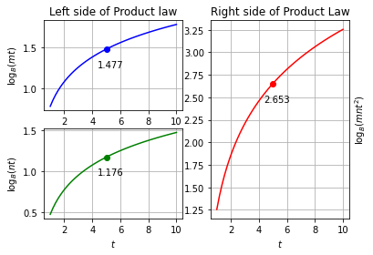
From the marked y-coordinates on the graph above, the points at \(\log(6t), \log(3t)\) and \(\log(18t^2)\) are at 1.477, 1.176 and 2.653 repectively.
This means that the left side of the equation equals the right side. Thus
Results
In the mathematical proof, we used the relationship between logarithms and exponents in order to derive the Product Law. Based on the values recorded during the graphical proof, we see that the left-hand side of the law is equivalent to sum of the two functions on the right-hand side.
Quotient Law
The next law we will be looking at is the Quotient Law. This is used when finding the difference of two logarithmic functions. The law states that
\(\log_{B}(x \div y)=\log_{B}x -\log_{B}y\).
An example
\(\log(1000 \div 100) = \log(1000) - \log(100)\) or equivalently
\(\log(10) = 1 = 3 -2.\)
Mathematical proof
Let’s create a proof of the Quotient law.
First, fix quantities \(x\) and \(y\) and define the values
\( p = \log_B x\) and \( q = \log_B y.\)
The equivalent exponential forms are
\(B^p= x\) and \(B^q = y\).
Divide these two equations to obtain:
\(B^p \div B^q = x \div y.\)
Using Exponential Law (2), the above equation is equivalent to:
\(B^{p-q}=x \div y.\)
Taking logs, we have
\(\log_{B}(B^{p-q}) = \log_B(x\div y) \) which becomes
\(p - q = \log_{B}(x \div y).\)
Recalling our definition of m,n this becomes
\(\log_B x - \log_B y = \log_B(x\div y),\)
which completes the proof of the Quotient Law.
Graphical Demonstration
As we know, the Quotient Law states: \(\log_{B}x+\log_{B}y = \log_{B}(x \times y).\)
To go about this, we introduce a parameter \(t\) that allows us to trace the graph of the logarithm function. We will also introduce two constant integers, \(m\) and \(n\).
We let \(x=mt\) and \(y=nt\) and set the base \(B\) to 10, abbreviating \(\log_{10}(x)\) as \(\log(x)\).
For these values of \(x\) and \(y\), the product law becomes
\(\log(mt)-\log(nt) = \log\left(\frac{mt}{nt}\right)\)
which reduces to:
\(\log(mt)-\log(nt) = \log\left(\frac{m}{n}\right)\)
For the graphical demonstration, we will graph the three terms in the above equation separately with respect to \(t\). When looking at a \(t\) value, the difference of the corresponding values of the functions on the left side of the equation should be equivalent to the function on the right side of the equation, thus providing a demonstration of the Quotient Law.
class QuotientLaw():

    # Create 2x2 sub plots
    gs = gridspec.GridSpec(2, 2)

    axis=5
    x=6
    y=3
    x_axis_bar = widgets.IntSlider(
        value=5,
        min=1,
        max=10,
        step=1,
        description='x',
        disabled=False,
        continuous_update=False,
        orientation='horizontal',
        readout=True,
        readout_format='d'
    )

    x_bar = widgets.IntSlider(
        value=x,
        min=1,
        max=10,
        step=1,
        description='$m$',
        disabled=False,
        continuous_update=False,
        orientation='horizontal',
        readout=True,
        readout_format='d'
    )

    y_bar = widgets.IntSlider(
        value=y,
        min=1,
        max=10,
        step=1,
        description='$n$',
        disabled=False,
        continuous_update=False,
        orientation='horizontal',
        readout=True,
        readout_format='d'
    )
    def create_graph():

        #########################################
        # Description: generates a graph in order to prove Quotient Law
        #
        # @Args: Inputs are for the variables shown in Quotient Law
        #        x-coordinate: based on a sliding bar in range 1-10
        #        M constant: based on a sliding bar in range 1-10
        #        N constant: based on a sliding bar in range 1-10
        #
        # @Return: graph for graphical proof as well as the y-coordinate corresponding to the graphed points
        #
        #########################################

        y_value=np.linspace(QuotientLaw.x/QuotientLaw.y,QuotientLaw.x/QuotientLaw.y)

        #Plot the 3 log functions from the left and right side of the Product Law
        ax1 = plt.subplot(QuotientLaw.gs[0, 0]) # row 0, col 0
        ax1.plot(x,Logarithm.log(QuotientLaw.x,base,x),'-b')
        p1=log(QuotientLaw.x*QuotientLaw.axis,base)
        ax1.plot(QuotientLaw.axis,p1,'ob')
        ax1.annotate('%1.3f' %p1,xy=(QuotientLaw.axis,p1),xytext=(-10,-20),textcoords='offset points')
        ax1.set_title('Left side of Quotient Law')
        plt.ylabel('$\log(m)$')
        plt.grid()

        ax2 = plt.subplot(QuotientLaw.gs[1, 0])
        ax2.plot(x,Logarithm.log(QuotientLaw.y,base,x),'-g')
        p2=log(QuotientLaw.y*QuotientLaw.axis,base)
        ax2.plot(QuotientLaw.axis,p2,'og')
        ax2.annotate('%1.3f' %p2,xy=(QuotientLaw.axis,p2),xytext=(-10,-20),textcoords='offset points')
        plt.ylabel('$\log(n)$')

        plt.xlabel('x')
        plt.grid()

        ax3 = plt.subplot(QuotientLaw.gs[:, 1])
        ax3.plot(x,Logarithm.log(1,base,y_value),'-r')
        p3=log(QuotientLaw.x/QuotientLaw.y,base)
        ax3.plot(QuotientLaw.axis,p3,'or')
        ax3.annotate('%1.3f' %p3,xy=(QuotientLaw.axis,p3),xytext=(-10,-20),textcoords='offset points')
        ax3.set_title('Right side of Quotient Law')
        plt.ylabel(r'$\log(\frac{m}{n})$')
        ax3.yaxis.set_label_position("right")
        plt.xlabel('x')
        plt.grid()
        plt.show()

        display(Latex('When $m$={1:2.0f} and $n$={2:2.0f}'.format(QuotientLaw.axis,QuotientLaw.x,QuotientLaw.y)))
        display(Latex('The y-coordinates at log({0:1.0f}$t$), log({1:1.0f}$t$) and log({2:1.0f}) are at {3:1.3f}, {4:1.3f} and {5:1.3f} repectively'.format(QuotientLaw.x,QuotientLaw.y,QuotientLaw.x/QuotientLaw.y,p1, p2, p3)))
        display(Latex('{0:1.3f}-{1:1.3f}={2:1.3f}'.format(p1,p2,p3)))
        display(Latex('thus'))
        display(Latex(r'$\log(m) - \log(n) = \log(\frac{m}{n})$'))

    def clear_display():
        clear_output(wait=True)
        display(QuotientLaw.x_bar)
        display(QuotientLaw.y_bar)
        display(QuotientLaw.x_axis_bar)
        QuotientLaw.create_graph()
        QuotientLaw.observe()

    def observe():
        QuotientLaw.x_axis_bar.observe(QuotientLaw.x_value, names='value')
        QuotientLaw.x_bar.observe(QuotientLaw.xv, names='value')
        QuotientLaw.y_bar.observe(QuotientLaw.yv, names='value')

    def x_value(value):
        QuotientLaw.axis=value['new']
        QuotientLaw.clear_display()

    def xv(value):
        QuotientLaw.x=value['new']
        QuotientLaw.clear_display()

    def yv(value):
        QuotientLaw.y=value['new']
        QuotientLaw.clear_display()

QuotientLaw.clear_display()
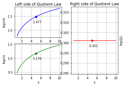
The y-coordinates at \( \log(6t), \log(3t)\) and \(\log(2)\) are at 1.477, 1.176 and 0.301 respectively
thus
Result
In the mathematical proof, we used the relationship between logarithms and exponents as well as exponential laws in order to derive the Quotient Law. When we look at the graphical demonstration, we see that the functions on the right hand side both resemble very similar curves. On the left hand side of the law, we can see that the function remains as a constant number. We also see that the left-hand side of the law is equivalent to the difference to the two functions on the right-hand side.
Power Law
The next law we will look at is power law. This is used in the case when there is an exponential power inside the logarithmic function. The law states that
\(\log_{B}(x^p)=p \times \log_B(x)\).
An example
\(\log(1000^2) = 2\log(1000) \) or equivalently
\(\log(1,000,000) = 6 = 2 \times 3.\)
Mathematical Proof
First we fix quantities \(x\) and \(p\) then define
\( m = \log_B (x^p).\)
The equivalent exponential form is
\(B^m=x^p\).
Bring each side of the equation to the power of \(1/p\) to obtain
\((B^m)^{\frac{1}{p}}=(x^p)^{\frac{1}{p}}.\)
By using Exponential Law (3), we can multiply the exponents to the one inside the brackets to get
\(B^{\frac{m}{p}}= x.\)
Apply the log function to both sides to get
\(\log_B(B^{\frac{m}{p}})=\log_B(x) \), resulting in
\(\frac{m}{p} = \log_B(x).\)
Multiply by \(p\) to obtain
\(m = p \times log_B(x),\) and recalling the definition of m, we have
\(\log_B(x^p) = p \times \log_B(x).\)
This completes the proof.
Graphical Demonstration
In this case, there is one function on each the left and right hand sides of the law. For this reason 2 functions will be graphed. Since they are theoretically be equivalent to each other, we can expect that the functions will be identical on the graph. If this is seen on the graph, we can validate Power Law.
As we know, the power Law states: \(\log_B(x^p) = p \times \log_B(x).\)
To go about this, we introduce a parameter \(t\) that allows us to trace the graph of the logarithm function. We will also introduce a constant interger, \(m\).
We let \(x=mt\) and set the base \(B\) to 10, abbreviating \(\log{10}(x)\) as \(\log(x)\).
For these values of \(x\) and \(y\), the product law becomes
\(\log_B(mt^p) = p \times \log_B(mt)\)
For the graphical demonstration, we will graph the three terms in the above equation separately with respect to \(t\). When looking at a \(t\) value, the function on the left side of the equation should be equivalent to the function on the right side of the equation, thus providing a demonstration of the power law.
class PowerLaw():
    # Create 2x2 sub plots
    gs = gridspec.GridSpec(1, 2)
    x=np.linspace(1,10)
    axis=5
    x=6
    p=2

    x_axis_bar = widgets.IntSlider(
        value=5,
        min=1,
        max=10,
        step=1,
        description='x',
        disabled=False,
        continuous_update=False,
        orientation='horizontal',
        readout=True,
        readout_format='d'
    )

    x_bar = widgets.IntSlider(
        value=x,
        min=1,
        max=10,
        step=1,
        description='$m$',
        disabled=False,
        continuous_update=False,
        orientation='horizontal',
        readout=True,
        readout_format='d'
    )


    p_bar = widgets.IntSlider(
        value=p,
        min=1,
        max=10,
        step=1,
        description='$p$',
        disabled=False,
        continuous_update=False,
        orientation='horizontal',
        readout=True,
        readout_format='d'
    )

    def create_graph():

        #########################################
        # Description: generates a graph in order to prove Power Law
        #
        # @Args: Inputs are for the variables shown in Power Law
        #        x-coordinate: based on a sliding bar in range 1-10
        #        M constant: based on a sliding bar in range 1-10
        #        N constant: based on a sliding bar in range 1-10
        #        R exponential constant: based on a sliding bar in range 1-10
        #
        # @Return: graph for graphical proof as well as the y-coordinate corresponding to the graphed points
        #
        #########################################

        #Plot the 3 log functions from the left and right side of the Product Law
        ax1 = plt.subplot(PowerLaw.gs[0,1]) # row 0, col 0
        ax1.plot(x,Logarithm.log_exp(PowerLaw.p,PowerLaw.x,base,x),'-g')
        p1=log((PowerLaw.x*PowerLaw.axis)**PowerLaw.p,base)
        ax1.plot(PowerLaw.axis,p1,'ob')
        ax1.annotate('%1.3f' %p1,xy=(PowerLaw.axis,p1),xytext=(-10,-20),textcoords='offset points')
        ax1.set_title('Right side of Power law')
        plt.ylabel('$y=\log_{B}(Mx)$')
        ax1.yaxis.set_label_position("right")
        plt.xlabel('x')
        plt.grid()

        ax2 = plt.subplot(PowerLaw.gs[0, 0])
        ax2.plot(x,Logarithm.constant_x_log(PowerLaw.p,PowerLaw.x,base,x),'-b')
        p2=PowerLaw.p*log(PowerLaw.x*PowerLaw.axis,base)
        ax2.plot(PowerLaw.axis,p2,'og')
        ax2.annotate('%1.3f' %p2,xy=(PowerLaw.axis,p2),xytext=(-10,-20),textcoords='offset points')
        plt.ylabel('$y=\log_{B}(Nx)$')
        ax2.yaxis.set_label_position("left")
        ax2.set_title('Left side of Power Law')
        plt.xlabel('x')
        plt.grid()
        plt.show()

        display(Latex('at $m$={0:1d} and $p$={1:1d}'.format(PowerLaw.x,PowerLaw.p)))
        display(Latex(r'We can see that the y-coordinates are labeled on the graph. At the points log(${0:1d}^{1:1d}x$) and {2:1d} $\times$ log({3:1d}$x$) the y-coordinates are {4:1.3f} and {5:1.3f} repectively'.format(PowerLaw.x,PowerLaw.p,PowerLaw.p,PowerLaw.x,p1,p2)))
        display(Latex('{0:1.3f}={1:1.3f}'.format(p1,p2)))

        display(Latex('thus'))
        display(Latex(r'$\log_{B}(x^p)=p \times \log_B(x)$'))

    def clear_display():
        clear_output(wait=True)
        display(PowerLaw.x_bar)
        display(PowerLaw.p_bar)
        display(PowerLaw.x_axis_bar)
        PowerLaw.create_graph()
        PowerLaw.observe()

    def observe():
        PowerLaw.x_axis_bar.observe(PowerLaw.x_value, names='value')
        PowerLaw.x_bar.observe(PowerLaw.xv, names='value')
        PowerLaw.p_bar.observe(PowerLaw.pv, names='value')

    def x_value(value):
        PowerLaw.axis=value['new']
        PowerLaw.clear_display()

    def xv(value):
        PowerLaw.x=value['new']
        PowerLaw.clear_display()


    def pv(value):
        PowerLaw.p=value['new']
        PowerLaw.clear_display()


PowerLaw.clear_display()
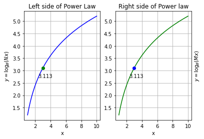
We can see that the y-coordinates are labeled on the graph. At the points \(\log(2^4x)\) and \( 4 \times \log(2x)\) the y-coordinates are 3.113 and 3.113 respectively.
thus
Results
The Mathematical proof shows that by first converting the logarithmic functions into exponents then using the exponential laws we can derive the power Law. When looking at the graph, we see that the function on the left-hand side are equavalent to the right-hand side.
Change of Base Rule
This rule is useful for changing the base of a logarithmic function which can be useful for proofs or comparing certain functions. The law states that:
\(\log_{B}(x)=\frac{\log_C(x)}{\log_C(B)}\)
An example
\(\log_8(64) = \frac{\log_2(64)}{\log_2(8)}\) or equivalently
\(2 = \frac{6}{3}.\)
Mathematical Proof
First we need to define a variable. In this case, we will use x.
\(\text{Let }x=\log_{B}(M)\)
When converting this to exponents by using basic logarithmic properties, we get:
\(B^x=M\)
\(\text{Next, is to apply } \log_N \text{ to both sides of the equation}\)
\(\log_N(B^x)=\log_N(M)\)
By Power Law (see above) this can be simplified to:
\(x\log_N(B)=\log_N(M)\)
Isolating for x:
\(x=\frac{\log_N(M)}{\log_N(B)}\)
After inputing the x value we defined earlier, we get:
\(\log_{B}(M)=\frac{\log_N(M)}{\log_N(B)}\)
Discussion
The change of base law says that
\(\log_B(x) = \frac{\log_C(x)}{\log_C(B)}.\)
Another way to write this is
\(\log_B(x) = \log_C(x)\times \log_B(C)).\) (Can you see why?)
The point is, the two functions \(\log_B(x), \log_C(x)\) are related by a proportionality constant, so we can write
For instance, the two functions \(\log_2(x)\) and \(\log_{10}(x)\) are the same, up to some constant \(k\). Perhaps you can explain why this constant is approximately \(10/3\). That is
Equivalently,
(Hint: this has something to do with our discussion of kilos in the first section of this notebook.)
Evidence
As it is hard to graph this function, as there is no good place to put \(x\), this function with be proved through evidence. We will plug numbers into each side of the equation to calculate the values obtained on each side of the law. Notice that changing the new base value has no affect on the final value.
class ChangeOfBase():

    #First set random variables
    M=5
    base=10
    new_base=5

    def create_graph():

        #########################################
        # Description: Plugs in numbers to prove Change of Base Rules
        #
        # @Args: Inputs are for the variables shown in Power Law
        #        M constant: based on a sliding bar in range 1-10
        #        base: based on a sliding bar in range 1-10
        #        new base: based on a sliding bar in range 1-10
        #
        # @Return: The corresponding value of each side of the equation which result after plugging in the numbers.
        #########################################


        p1=log(ChangeOfBase.M,ChangeOfBase.base)
        p2=log(ChangeOfBase.M,ChangeOfBase.new_base)/ log(ChangeOfBase.base,ChangeOfBase.new_base)

        display(Latex('On the left hand side $\log_B(M)$ = {0:1.3f}.'.format(p1)))
        display(Latex(r'On the right hand side is $\log_C(M) \div \log_C(B)$ = {0:1.3f}.'.format(p2)))
        display(Latex('{0:1.3f} = {1:1.3f}'.format(p1,p2)))
        display(Latex('thus'))
        display(Latex(r'$\log_{B}(M) = \frac{\log_C(M)}{\log_C(B)}$'))

    def clear_display():
        clear_output(wait=True)
        display(m_box)
        display(base_box)
        display(new_base_box)
        ChangeOfBase.create_graph()

    def xv(value):
        ChangeOfBase.axis=value['new']
        ChangeOfBase.clear_display()

    def Mv(value):
        ChangeOfBase.M=value['new']
        ChangeOfBase.clear_display()

    def Basev(value):
        ChangeOfBase.base=value['new']
        ChangeOfBase.clear_display()

    def New_basev(value):
        ChangeOfBase.new_base=value['new']
        ChangeOfBase.clear_display()

M_bar = widgets.IntSlider(
    value=ChangeOfBase.M,
    min=1,
    max=10,
    step=1,
    disabled=False,
    continuous_update=False,
    orientation='horizontal',
    readout=True,
    readout_format='d'
)

m_box = HBox([Label('M value'), M_bar])

base_bar = widgets.IntSlider(
    value=ChangeOfBase.base,
    min=2,
    max=10,
    step=1,
    disabled=False,
    continuous_update=False,
    orientation='horizontal',
    readout=True,
    readout_format='d'
)

base_box = HBox([Label('Original base value'), base_bar])

new_base_bar = widgets.IntSlider(
    value=ChangeOfBase.new_base,
    min=2,
    max=10,
    step=1,
    disabled=False,
    continuous_update=False,
    orientation='horizontal',
    readout=True,
    readout_format='d'
)

new_base_box = HBox([Label('New base value'), new_base_bar])

ChangeOfBase.clear_display()
M_bar.observe(ChangeOfBase.Mv, names='value')
base_bar.observe(ChangeOfBase.Basev, names='value')
new_base_bar.observe(ChangeOfBase.New_basev, names='value')
thus
Results
The mathematical proof uses the relationship between logarithms and exponents in order to change the value of the base and thus derive the rule. When plugging numbers into the rule, we can see that the left hand side of the equation is always equal to the right hand side, regardless of the numbers that are plugged in. By these 2 proofs, we can confirm the changing base rule.
Examples
1. Simplify the following equation, then solve for \(x\)
\( 3^{\log(x)}3^{\log(x)}\)
Using Exponential Law (1), we can get:
\(3^{\log(x)+\log(x)}\)
This is simplified to:
\(3^{2\log(x)}\)
Using Power law, we know \(2\log(x)=\log(x^2)\). From this identity, we simplify the expression to:
\(3^{\log(x^2)}\)
To solve for \(x\), we need to first note that \(3 = 10^{\log 3}.\) So we can continue with
\( 3^{\log(x^2)} = 10^{\log 3 \log x^2} = 10^{\log x^{2\log 3}} = x^{2\log 3} = x^{\log(9)}.\)
Thus, we can say:
\(x^{\log(9)} \approx x^{.954}\)
2. \(\text{Simplify the expression: } 2\log(x) - \frac{\log(z)}{2} + 3\log(y)\)
Next, we will apply Power Law on each term. While keeping in mind that \(z^{\frac{1}{2}}=\sqrt{z}\), we can simplify this equation to:
\(\log\left(x^2\right) - \log(\sqrt{z})+\log(y^3)\)
We can apply both Quotient and Product Law to this equation. This will result in the final simplified form of:
3. Solve for x \( 2^{(x-2)}=2^x -2 \)
Using Exponent Law (2) reguarding the division of exponents, we can come up with the equivalent equation:
\(\frac{2^x}{2^2}=2^x-2\)
The next step is to complete simple algebra. We can put all of the \(2^x\) terms on the same side to isolate for x.
The intermediate step is:
\(2^x=4(2^x-2)\)
When we put all of the \(2^x\) terms on the same side, we get:\(-3(2^x)=-8\)
which becomes:
\(2^x = \frac{8}{3}\)
Since we know, \(\log_2(2)=1\), we can apply \(\log_2\) onto both sides. We get:
\(\log_2(2^x)=\log_2\left(\frac{8}{3}\right)\)
Using Power Law, \(\log_2(2^x)\) is equivalent to \( x\log_22\) where \(\log_22 = 1\). Thus:
Conclusion
When analysing each of the 5 functions in mathematical and graphical ways, that each of these 5 laws can be proven and validated. This creates shortcuts to make it easier to simplify and analyze more complex functions.
