

![]()
%%html

<script>
  function code_toggle() {
    if (code_shown){
      $('div.input').hide('500');
      $('#toggleButton').val('Show Code')
    } else {
      $('div.input').show('500');
      $('#toggleButton').val('Hide Code')
    }
    code_shown = !code_shown
  }

  $( document ).ready(function(){
    code_shown=false;
    $('div.input').hide()
  });
</script>
<p> Code is hidden for ease of viewing. Click the Show/Hide button to see. </>
<form action="javascript:code_toggle()"><input type="submit" id="toggleButton" value="Show Code"></form>
Code is hidden for ease of viewing. Click the Show/Hide button to see.
import numpy as np
import matplotlib.pyplot as plt
from IPython.display import display, Math, Latex, HTML, clear_output, Markdown, Javascript
import ipywidgets as widgets
from ipywidgets import interact, interact_manual, FloatSlider, IntSlider, interactive, Layout
from traitlets import traitlets
import warnings


import plotly as py
import plotly.graph_objs as go
from plotly.offline import download_plotlyjs, init_notebook_mode, plot, iplot
init_notebook_mode(connected=True)
Root Finding Algorithms

Introduction
In this notebook you will gain an understanding of basic root-finding algorithms and their implementation. This topic is introduced with the goal of easing you into numerical solutions to mathematical problems. We will outline the advantages and disadvantages of solving a problem numerically rather than analytically. At the end of the notebook there will be example problems, in which you have the opportunity to implement these methods, yielding a broader understanding of their applicability and power.
Necessary background:
Be able to factor quadratic polynomials
Understand basic python syntax
Read, graph, and analyze functions
Rudimentary algebra
In this Notebook you will see examples of code to perform some basic root-finding algorithms. You will not be required to know how the code works or need to write any yourself. Nevertheless, you will be encouraged to manipulate some of the lines in order to input a function of your choice, but that is all. The pieces of code and algorithms can be simply thought of as tools to execute the task you want them to perform, and only running them will be a necessary to accomplish this task. Although the coding isn’t required, I strongly encourage you to try to understand how and why it works.
For a warm-up, we have created an exercise for you to determine the intervals on which a polynomial is \(>\) 0. A first approach to this problem would be to find the roots of the polynomial and then analyze the behaviour in between these roots. We recommend converting the function into a form that you can graph in order to determine the behaviour on either side of the roots. Think about the possible forms of the graph, i.e. concavity, convexity, and what this tells you about the intervals where the function is positive. This type of analytical thinking will help further along in the notebook.
Given a polynomial of order \(\leq\) 3, find where the function is \(>\) 0. Below is simply a method of approaching this problem, not necessarily the best or most effective. There are many ways one can go about this, each offering a different insight or understanding. Find what works best for you and try to understand why you used this method (is it visual? is it solely algebraic? did you manipulate the function?).
Example:
Find the interval on which \(f(x) = x^2 - 3x +2 > 0\).
Solve for roots:
\(f(x) = (x-1)(x-2)\)
Using an inequality approach, if I picked a point, \(c\) in the interval \((1,2)\), then (c-1)> 0 and (c-2)< 0. Therefore, our function evaluated at this point:
\(f(c)=(c-1)(c-2) < 0\).
We can deduce, by knowing the shape of a parabola, that the interval on which \(f(x)>0\) is \(x = (-\infty,1)\cup(2,\infty)\)
By picking a point in between the roots we quickly found whether the function was concave up or down. Knowing what the graph of a parabola looks like, this quickly told us where the function was positive.
Given a polynomial of order 2 or 3, find where the function \(>\) 0. Try polynomials of 2nd order first and then 3rd for more of a challenge. Below, we will provide some algorithms that will make finding the roots of a third (or higher) order polynomial much less tedious.
Please input your answer in interval notation, using “U” for the union of intervals. Press Enter after typing your response.
For \(\infty\) type infinity
If the function is nowhere \( > 0\), then type “Nowhere”
I recommend trying the exercise for a polynomial of order two, reviewing the content of the notebook and then trying for polynomials of order 3. Input answer in interval notation (i.e. (-4,-1)U(5,infinity) ):
def find_interval(poly_order):
    poly_order = int(poly_order)
    if poly_order > 3:
        display('Order of polynomial must be less than or equal to 3')
        display('Provide order of polynomial:')

    if poly_order == 3:
        C = np.random.randint(-5,5,poly_order)
        C1 = -1*np.sum(C)
        C2 = C[0]*C[1] + C[2]*(C[0]+C[1])
        C3 = -1*C[0]*C[1]*C[2]
        C11=C1
        C22=C2
        C33=C3
        display("Find the interval where P(x) > 0 :")
        if C1>0:
            str1 = '+' + str(C11) + 'x^2'
        elif C1== 0:
            str1 = ''
        else:
            str1=  str(C11) + 'x^2'
        if C2>0:
            str2 = '+' + str(C22) + 'x'
        elif C2== 0:
            str2=''
        else:
            str2= str(C22) + 'x'
        if C3>0:
            str3 = '+' + str(C33)
        elif C3== 0:
            str3=''
        else:
            str3= str(C33)

        a = "P(x)= x^3" + str1 + str2 + str3

        display(Math(a))

        def poly(x):
            return x**3 + C1*x**2 + C2*x + C3

    if poly_order == 2:
        C = np.random.randint(-5,5,poly_order)
        C1 = -1*np.sum(C)
        C2 = C[0]*C[1]
        C11=C1
        C22=C2
        if C1>0:
            str1 = '+' + str(C11) + 'x'
        elif C1== 0:
            str1 = ''
        else:
            str1=  str(C11) + 'x'
        if C2>0:
            str2 = '+' + str(C22)
        elif C2== 0:
            str2=''
        else:
            str2= str(C22)
        display('Find the interval where P(x) > 0  :')
        a = 'P(x) = x^2 ' + str1 + str2
        display(Math(a))
        def poly(x):
            return x**2 + C1*x + C2

    Max = max(C)
    Min = min(C)
    M = [Min, Max]
    V = np.sort(C)
    eps = 0.1

    if poly_order ==3:
        v = V[1]
        if Max == Min and poly(Max +eps) > 0:
                          interval = '('+str(Max)+',infinity)' #One single root, increasing
        if Max == Min and poly(Max +eps) < 0:
                          interval = '(-infinity,' + str( Max)+')' #One single root, decreasing

        if poly(Max + eps) >0:
#         interval = '(' + str(Max) + ', infinity)'
            if v !=  Max and v!= Min:
                          interval = '('+str(Min) + ',' + str(v) + ')U(' + str(Max) + ',infinity)'
            if v == Max:
                          interval = '(' + str(Min) + ', infinity)'
            if v== Min:
                          interval = '(' + str(Max) + ', infinity)'

        if poly(Max + eps) <0:
#         interval = '(-infinty,' + str(Min) + ')'
            if v != Max and v != Min:
                          interval = '(-inifinity,' + str(Min) + 'U('+str(v) + ','+str(Max) + ')'
            if v == Max:
                          interval = '(-infinity,' + str( Max) + ')'
            if v == Min:
                          interval = '(-infinity,' + str(Min) + ')'

    if poly_order == 2:
            if Max == Min and poly(Max+eps)>0:
                interval = '(-infinity,'+str(Min)+')U('+str(Min)+',infinity)' #one root, convex
            elif poly(Max+eps)<0:
                interval = '('+str(Min)+','+str(Max)+')' #Two distinct roots, Concave
            elif poly(Max + eps)>0:
                interval = '(-infinity,'+str(Min)+')U(' + str(Max)+',infinity)' #Two distinct roots, convex
            else:
                interval = 'Nowhere' #one root, concave

    x = np.linspace(-100,100,10000)
    p = poly(x)

    return interval, p


def check_answer(answer,interval,y):

    answer = answer.replace(" ","")

    if answer == "":
        display("Please be sure to press enter after submitting your answer.")
    else:
        if answer != interval:
            display("That's not quite right, try again.")
        if answer == interval:

            display("Correct! Here's a visualization of the solution:")
            x1=np.linspace(-100,100,10000)
            trace = go.Scatter(
                x = x1,
                y = y
            )
            layout = go.Layout(
                xaxis = dict(
                    title='x',
                    titlefont=dict(
                    family='Arial, serif',
                    size=18,
                    color='black'),
                    range = [-10,10],
                    ticks='inside',
                    tick0=0,
                    dtick=1
                ),
                yaxis = dict(
                    title='P(x)',
                    titlefont=dict(
                    family='Arial, serif',
                    size=18,
                    color='black'),
                    range = [-10,10],
                    ticks='inside',
                    tick0=0,
                    dtick=1
                ),
            )

            data = [trace]

            fig = go.Figure(data=data, layout=layout)
            iplot(fig)

    return


text2 = widgets.Text(disabled = False, placeholder = 'Enter Interval')
out2 = widgets.Text(disabled  = True, value = None)
text3 = widgets.Text(disabled = False, placeholder = 'Enter Interval')
out3 = widgets.Text(disabled  = True, value = None)

def bind_to_out2(sender):
    out2.value = text2.value
    return out2.value

text2.on_submit(bind_to_out2)

def bind_to_out3(sender):
    out3.value = text3.value
    return out3.value

text3.on_submit(bind_to_out3)

button2 = widgets.Button(description="Attempt Exercise (order 2)",
                         layout = Layout(width='30%', height='60px'),
                         button_style = 'info'
                        )
button3 = widgets.Button(description="Attempt Exercise (order 3)",
                         layout = Layout(width='30%', height='60px'),
                         button_style = 'info'
                        )
check_button2 = widgets.Button(description="Check your answer",
                              layout = Layout(width='30%', height='60px'),
                              button_style = 'info'
                             )
check_button3 = widgets.Button(description="Check your answer",
                              layout = Layout(width='30%', height='60px'),
                              button_style = 'info'
                             )

H1 = widgets.HBox([button2, button3])
display(H1)

def on_button_clicked2(b):
    text2.value = ""
    clear_output()
    display(H1)
    display(Javascript('IPython.notebook.execute_cell_range(IPython.notebook.get_selected_index()+0,IPython.notebook.get_selected_index()+1)'))
    display(Javascript('IPython.notebook.execute_cell_range(IPython.notebook.get_selected_index()+1,IPython.notebook.get_selected_index()+2)'))

button2.on_click(on_button_clicked2)


def on_button_clicked3(b):
    text3.value = ""
    clear_output()
    display(H1)
    #Rerun this cell to avoid the multiple outputs
    display(Javascript('IPython.notebook.execute_cell_range(IPython.notebook.get_selected_index()+0,IPython.notebook.get_selected_index()+1)'))
    display(Javascript('IPython.notebook.execute_cell_range(IPython.notebook.get_selected_index()+2, IPython.notebook.get_selected_index()+3)'))

button3.on_click(on_button_clicked3)
clear_output()
interval2, y2 = find_interval(2)

display(text2)
display(check_button2)

def check2(b):
    check_answer(out2.value,interval2,y2)


check_button2.on_click(check2)
'Find the interval where P(x) > 0 :'
interval3, y3 = find_interval(3)
display(text3)
display(check_button3)

def check3(b):
    check_answer(out3.value,interval3,y3)

check_button3.on_click(check3)
'Find the interval where P(x) > 0 :'
Analytic vs. Numerical Solutions
Below we will outline the differences, pros and cons and methods of analytic vs. numerical solutions within the context of root finding. By solving for the roots of the polynomial and analyzing the graph of the function, you were able to explicitly determine an answer to the question posed. This is the benefit of these analytic expressions; they give you a nice and clear explicit answer. It is often the case that we can derive analytic solutions to simpler, well-posed problems. Now, what if the problem is not so well-posed? What if our analytic approach becomes way too complex or tedious? How would you approach this problem without finding zeroes? What if the polynomial is of \(n^{\rm th}\) order? For these cases we turn to a numerical approach, alleviating the work load and attaining the same end goal, but often with less accuracy.
Next we will walk you through different ways to approach this problem, and more complex problems of the same flavour, numerically. You will gain some insight into the implementation and benefit of numerical solutions while developing some basic skills in Python and numerical analysis.
Inspection
In order to answer the question, “On what interval(s) is \( f(x) > 0?\)”, you probably found the roots of the polynomial and looked at the behaviour of the graph in between these roots. This can be done for nice polynomials with integer coefficients and a low-order, but becomes increasingly difficult the more terms there are and the less simple the polynomials starts looking. Nevertheless, your initial approach to this problem can still be taken, i.e. find the roots and analyze the behaviour in between these roots in order to determine where \(f(x)>\) 0. Below we will discuss some algorithms used to determine roots of a polynomial.
Take, for instance, the polynomial: \(f(x) = x^3 -\frac{7}{9}x^2 - \frac{1}{4}x+\frac{7}{36}\)
A great advantage of utilizing a numerical approach is that it allows for quick ways to approximate a solution. This is useful if the amount of error is negligible and all one is looking for is an estimation. A quick way to get an estimation for our solution in question is simply to plot \(f(x)\). This is similar to what you would do on your graphing calculator, now just on the computer using code! If you would like to get started plotting with python, the best place to start is with matplotlib. It’s quick to learn, if you know basic python syntax, and there are tons of internet resources to explore its capabilities and debug problems. For extensive documentation and functionality of the matplotlib library see https://matplotlib.org/. Click on plot function to inspect \(f(x)\) above.
button = widgets.Button(description="Plot Function",
                        layout = Layout(width='30%', height='60px'),
                        button_style = 'info'
                       )
display(button)
def on_button_clicked(b):

    x = np.linspace(-50,50,1000)
    y = x**3 - (7/9)*x**2 - (1/4)*x + 7/36
    trace = go.Scatter(
        x = x,
        y = y
    )
    layout = go.Layout(
        xaxis = dict(
            title='x',
            titlefont=dict(
            family='Arial, serif',
            size=18,
            color='black'),
            showticklabels=True,
            tickangle=0,
            range = [-1,1],
            ticks='outside',
            tick0=0,
            dtick=1
        ),
        yaxis = dict(
            title='P(x)',
            titlefont=dict(
            family='Arial, serif',
            size=18,
            color='black'),
            range = [-1,1],
            ticks='outside',
            tick0=0,
            dtick=1
        ),
    )

    data = [trace]

    fig = go.Figure(data=data, layout=layout)

    iplot(fig)

button.on_click(on_button_clicked)
on_button_clicked(0)
Purely by inspection, we were able to observe where the roots of this function lie: \(x \approx -\frac{1}{2},\frac{1}{2},\frac{3}{4}\). This was a nice and clean numerical solution to a problem that would’ve been much more difficult to solve analytically. Although this may seem convenient and albeit simple, this estimation approach is primitive. It is rare that a problem would ever require this simple of a solution, but nonetheless we found the roots of the polynomial. By simply graphing the solution, we were also able to see easily where the function was greater than zero.
Here we will provide an exercise to determine roots of a function based on arbitrary parameters and visualize how a graph of the function changes for different values of these parameters. Learning outcomes:
You will understand how arbitrary parameters change the graph of a quadratic polynomial function
Understand how to determine the roots given arbitrary values
See how the roots change under changing the values of the parameter
First we provide the steps to derive the famous “Quadratic Formula”, try following them on your own, click Show Answer to see the answer.
Starting with an arbitrary polynomial, \(P(x) = ax^2 + bx + c\), where \(a \ne 0\):
Set \(P(x) = 0\).
Complete the square.
Rearrange the equation, isolating “\(x\)”.
button = widgets.Button(description="Show Answer",
                        layout = Layout(width='30%', height='60px'),
                         button_style = 'info'
                       )
display(button)

def on_button_clicked(b):
    display(Markdown('$ P(x) = ax^2 + bx + c = 0$ </br> </br> \
    Complete the square, first dividing by a:</br> </br> \
    $\\frac{P(x)}{a} = (x+\\frac{b}{2a})^2 + \\frac{c}{a} - \\frac{b^2}{4a}= 0$ </br> </br>\
    Rearrange for $x$: </br> </br> \
    $(x+\\frac{b}{2a})^2 = \\frac{b^2}{4a^2} -\\frac{c}{a} = \\frac{b^2 - 4ac}{4a^2}$ \
    $\Rightarrow x+\\frac{b}{2a} = \pm \\frac{\sqrt{b^2-4ac}}{\sqrt{4a^2}}$ </br> \
    $\Rightarrow x = -\\frac{b}{2a} \pm \\frac{\sqrt{b^2-4ac}}{2a}$'))
    button_clicked = 1
button.on_click(on_button_clicked)
A potential use of inspection would be our initial exercise: “Find the intervals where \(f(x) > 0\) “. The next cell has been left for you to input the values \((a,b,c,d)\) for a third order polynomial in the form \(f(x) = ax^3 + bx^2 + cx + d\) the function that our first exercise output, see if you can use inspection to obtain the correct interval. Also, by setting \(a\) to zero, see observe how the roots change for a quadratic function. Think about how changing these parameters changes the roots obtained from the “Quadratic formula” (e.g. what does increasing the value of \(c\) do?). Press the “Plot Function” to start this exercise.
#function to graph third order polynomial with given inputs:
def plot3(a,b,c,d):
    x = np.linspace(-50,50,1000)
    y = a*x**3 + b*x**2 + c*x + d
    trace = go.Scatter(
        x = x,
        y = y
    )
    layout = go.Layout(
        xaxis = dict(
            title='x',
            titlefont=dict(
            family='Arial, serif',
            size=18,
            color='black'),
            showticklabels=True,
            tickangle=0,
            range = [-15,15],
            ticks='outside',
            tick0=0,
            dtick=1
        ),
        yaxis = dict(
            title='P(x)',
            titlefont=dict(
            family='Arial, serif',
            size=18,
            color='black'),
            range = [-25,25],
            ticks='outside',
            tick0=0,
            dtick=5
        ),
    )

    data = [trace]

    fig = go.Figure(data=data, layout=layout)

    iplot(fig)

    return

a = widgets.IntSlider(
    value=1,
    min=-10,
    max=10,
    step=1.0,
    description=r'$a$:',
    disabled=False
)
b = widgets.IntSlider(
    value=1,
    min=-10,
    max=10,
    description=r'$b$:',
    disabled=False
)
c = widgets.IntSlider(
    value=1,
    min=-10,
    max=10,
    description=r'$c$:',
    disabled=False
)
d = widgets.IntSlider(
    value=1,
    min=-10,
    max=10,
    description=r'$d$:',
    disabled=False
)
H = widgets.HBox([a,b,c,d])

abc = widgets.interactive_output(plot3, {'a': a, 'b': b, 'c': c, 'd': d})


button = widgets.Button(description="Plot Function",
                        layout = Layout(width='30%', height='60px'),
                         button_style = 'info'
                       )
display(button)
def on_button_clicked(b):

    button_clicked = display(abc,H)
    d.value = 0 #this is so it plots, widget has to change value in order to observe change

button.on_click(on_button_clicked)

on_button_clicked(0)
We will now proceed into some algorithmic numerical methods for root finding. These methods are useful as they can be easily integrated into a computer program. These are some of the more basic methods but they are often combined with each other, or with other methods, for more robust applications that require greater accuracy and less processing time. We first introduce how to use these methods analytically, then introduce a sketch of the code in python syntax. The analytic approach provides a means of solving the problem, while the numerical approach speeds the calculations up. Combining the two approaches provides insight into potential problems that arise in the computations and how to remedy them.
Bisection Method
The bisection method is a simple algorithm to quickly find an approximation for a root. The basic idea of the method is to initially take an interval, \([a,b]\) over which a function \(f\) is continuous, such that \(f(a)\) and \(f(b)\) have different signs (so you know that there is a root in between). We then split the interval into two and check the new endpoints of each subinterval. Let \(c = (a+b)/2\) be the midpoint of the interval. If the function values at the endpoints of one of these two subintervals have identical signs (that is, if \(f(a)\) and \(f(c)\) have the same signs or \(f(b)\) and \(f(c)\) have the same signs) then this subinterval is discarded, knowing that a root must lie within the other subinterval. Note that a root could also exist within the other interval but it is not guaranteed. We then divide this subinterval into two and repeat the same analysis on it. Eventually, up to an accuracy that we are happy with, we will have a small interval within which a root is found.
Analytical Approach
Try this method, analytically, for \(f(x)= x^2-4\) and the initial interval \([0,5]\). Try three iterations of the algorithm, and see the accuracy you obtain. Would you be happy with this accuracy? Do you feel this was quick enough? Click “Show Answer” to see the calculations, after you have done so yourself of course…
button = widgets.Button(description="Show Answer",
                        layout = Layout(width='30%', height='60px'),
                         button_style = 'info'
                       )
display(button)

def on_button_clicked(b):
    display(Markdown('Firstly, $f(0) = -4$ and $\\rm f(5) = 21$, which have opposite signs, so this is a valid interval to start with. </br> </br> \
    Split the interval in two: $c_1 = \\frac{0+5}{2} = 2.5$. </br> </br> \
    Check the sign of the function for on each subinterval endpoint (i.e. check the sign of $f(c)$):  $f(2.5) = 2.25$, therefore our new interval is $[0,2.5]$.</br> </br> \
    Split interval again and check signs of function at the middle: $c_2 = \\frac{2.5+0}{2} = 1.75$ , $f(1.75) = -0.9375$ </br> </br> \
    $\Rightarrow$ new interval is $[1.75,2.5]$, $c_3 = \\frac{1.75+2.5}{2}$, $f(c_3) = 0.515625$, new interval = $[1.75,2.125]$ </br> </br> \
    root is approximately $c_4 = \\frac{1.75 + 2.125}{2} = 1.9375$ </br> </br> \
    Percent error: $\\frac{2-1.9375}{2} x 100\% = 3.125 \%$'))
    button_clicked = 1
button.on_click(on_button_clicked)
We can clearly see that the method is somewhat slow and really good accuracy is hard to achieve. Nevertheless, it narrowed down our intervals and gave us a fairly good approximation to the root. What about the other root at \(x = -2\), how could we have obtained this root? Well, with a different set of initial conditions (our initial interval). The initial conditions play a very important role for this method as they can yield different results for a root. Try this same procedure, now instead with \([-5,0]\) as your starting point. Your answer after each iteration should be the same, except with a different sign.
This serves to illustrate a flaw in a lot of root finding algorithms; the sensitivity to the initial guess. Many of these algorithms require a good educated guess to work properly. Moreover, the algorithm can only determine one root for each initial guess, which is another disadvantage.
Numerical Approach
Specify the initial interval and the tolerance (accuracy) that you would like to achieve:
x0 = -1
x1 = 1
tol = 0.01
Define the function you would like to find the root for:
def f(x):
    return x**3 - (7/9)*x**2 -(1/4)*x + 7/36
This function can accept a single number or a whole list of numbers: it returns an output that applies a function to the given number or every number in the given list. Now we can begin the algorithm. First we set up the initial conditions:
c =(x1 + x0)/2  #where c is the mid-point, as defined in the analytical solution
if (f(x0) > 0 and f(x1) > 0) or (f(x0) < 0 and f(x1) < 0):
    print('Pick new initial conditions') #The Bisection method does not apply for these cases
else:
    while f(c) > tol:  #run the loop until your tolerance is satisfied

        if f(c) == 0:
            break   # you have found a root; break out of the while loop
        if sign(f(c)) == sign(f(x0)):
            x0 = c #Interval [x0,c] does not necessarily have a root; x0 is set to c
        if sign(f(c)) == sign(f(x1)):
            x1 = c #Interval [c,x1] does not necessarily have root; x1 is set to c

        c = (x1+x0)/2  # update the value of c, based on the current values of x0 and x1
    print(c)
What does the while statement do?
The statement
while f(c) > tol:
deserves some unpacking. This is what is known as a while loop, and is an essential tool used in programming. The indented code written after the colon will be executed until the conditional statement \(f(c) > \rm tol\) doesn’t hold anymore. Here is a visual interpretation of this process:
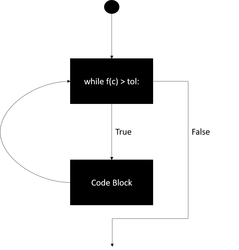
Common errors that occur:
Infinite loop: this is probably the most common error that occurs with a while loop. This happens if the statement is always true, i.e. the code block never makes the conditional statement false.
Loop is not entered: This occurs if the conditional statement is not initially satisfied. This depends on our initial guess for \([x_0,x_1]\).
The next cell is an illustration of how one could write a piece of code to execute this algorithm. The default initial conditions are \(x_0 = -1\), \(x_1 = 1\). The same code is included in the cell afterwards, if you would like to change the inital conditions or the function itself, press the “show code” to manipulate the algorithm.
#Bisection Method algorithm


#Specify the initial interval
x0 = -1
x1 = 1

#Specify tolerance (accuracy) you want:
tol = 0.01

#Function (of your choice) we will use our function from before:
def f(x):
    return x**3 - (7/9)*x**2 -(1/4)*x + 7/36

#Defining a sign function
def sign(x):
    if x < 0:
        sign = 0
    if x >= 0:
        sign = 1
    return sign

#Bisection method algorithm
c = (x1+x0)/2  #Midpoint
if (f(x0) > 0 and f(x1) > 0) or (f(x0) < 0 and f(x1) < 0):
    print('Pick new initial conditions') #The Bisection method does not apply for these cases
else:
    while f(c) > tol:  #run the loop until your tolerance is satisfied
        c = (x1+x0)/2
        if f(c) == 0:
            break   # you have found a root; break out of the while loop
        if sign(f(c)) == sign(f(x0)):
            x0 = c #Interval [x0,c] does not necessarily have a root; x0 is set to c
        if sign(f(c))== sign(f(x1)):
            x1 = c #Interval [c,x1] does not necessarily have root; x1 is set to c
        root = (x1+x0)/2
    display('Root =  ' + str(round(root,4)))
'Root = -0.75'
Secant Method
Here we will walk you through a root-finding algorithm known as the secant method which provides quick approximations of roots. For a quick review or another reference of this method and other root finding algorithms, please see https://en.wikipedia.org/wiki/Root-finding_algorithm.
In this section of the tutorial we will demonstrate the basics of the method and walk you through some of the elementary steps you would need to write a root-finding algorithm implementing the secant method yourself.
Analytical approach
The secant method employs successive operations, known as iterations, of finding the root of a secant line of a function \(f(x)\).
A secant line can thought of as a line which intersects a curve at two points. Given the domain \([a,b]\) and a continuous function \( f:[a,b] \mapsto \mathbb{R}\), take two points \( x_0, x_1 \in [a,b]\). The secant line between these two points, in slope-intercept form is given as:
The next step in the algorithm is to find the \(x\) intercept of this line:
This point now becomes our next endpoint, i.e.:
We now iterate this algorithm, applying the same process successively, until our algorithm yields a value \(f(x_n) \approx 0\) after n iterations.
Numerical Approach
The algorithm to implement the secant method is given as follows.
#same function as for the bisection method
def f(x):
    return x**3 - (7/9)*x**2 -(1/4)*x + 7/36  #Function to employ algorithm on

#initial conditions
n = 20 #number of iterations you want to use

for i in range(1,n):
    x2 = x1-f(x1)*((x1-x0)/(f(x1)-f(x0))) #equivalent to what we had defined analytically
    x0 = x1  #update the values
    x1 = x2  #update

print(x1)
    break
What does the for statement do?
The statement
for i in range(1,n):
also deserves some explanation. This is another essential programming tool known as the for loop. Within the for statement, the indented code block is executed, then the next iteration of the loop is performed, in our case \(i \mapsto i+1\), and this continues until all iterations are done (\(i = n\)). It provides a means of counting or iterating through a process. In our case these are the iterations of the secant method.
Note: The print(x1) statement is outside of the indented block. This means that x1 is printed after the loop has finished. If the statement were included within the block, then x1 would be every time (how many times would x1 be printed?).
Below is a visualization of the algorithm at work. Input the initial values of \(x_0\) and \(x_1\) below and press “Iterate” to see how the algorithm searches for the roots of the same function used in the “Inspection” example. This will give you a sense how this algorithm works and the problems it may run into. Reset the cell by pressing restart and playing around with different initial conditions to gain a better sense of how the algorithm works. Does it seem faster than the bisection method? How many iterations are required until it converges to the solution with the accuracy you wanted? Did it even converge? Notice how different initial guesses can make the algorithm converge to different roots.
Try working through the algorithm analytically, on paper with a function of your choice, beforehand. See how fast you can obtain a root and to what accuracy.
# Secant method visualization
#First we define our arbitrary function
x = np.linspace(-10,10,10000)
f = x**3 - (7/9)*x**2 -(1/4)*x + 7/36 #Underlying plot

def func(x):
    return x**3 - (7/9)*x**2 -(1/4)*x + 7/36  #Function to employ algorithm on

class LoadedButton(widgets.Button):
    #A button that can holds a value as a attribute.

    def __init__(self, value=None, *args, **kwargs):
        super(LoadedButton, self).__init__(*args, **kwargs)
        # Create the value attribute.
        self.add_traits(value=traitlets.Any(value))


def secantmethod(x0,x1,n,tol):

    if str.isdigit(x0) == False or str.isdigit(x1) == False or str.isdigit(tol) == False:
        print("Please input a number")
    else:
        if x0 and x1 != None:
            x0.replace(" ","")
            x1.replace(" ","")
            tol.replace(" ","")
            x0 = np.array(x0).astype(np.float)
            x1 = np.array(x1).astype(np.float)
            tol = np.array(tol).astype(np.float)

            for i in range (1,n):
                x2 = x1-func(x1)*((x1-x0)/(func(x1)-func(x0)))
                x0 = x1
                x1 = x2
                if abs(x1-x0)< tol:

                    display(Markdown("Secant method has provided the root to within the specified tolerance"))
                    display(Markdown('Root = '+ str(round(x1,4))))
                    break

    return x0, x1


x0s_in = widgets.Text(placeholder = "Enter a Value")
x0s_out = widgets.Text(value = None, disabled = True)
x1s_in = widgets.Text(placeholder = "Enter a Value")
x1s_out = widgets.Text(value = None, disabled = True)
tols_in = widgets.Text(placeholder = "Enter a Value")
tols_out = widgets.Text(value = None, disabled = True)

def bind_x0(sender):
    x0s_out.value = x0s_in.value
    return x0s_out.value
def bind_x1(sender):
    x1s_out.value = x1s_in.value
    return x1s_out.value
def bind_tol(sender):
    tols_out.value = tols_in.value
    return tols_out.value

x1s_in.on_submit(bind_x1)
x0s_in.on_submit(bind_x0)
tols_in.on_submit(bind_tol)

lb = LoadedButton(description="Iterate", value=0,
                  layout = Layout(width='30%', height='60px'),
                  button_style = 'info'
                 )

restart_button = widgets.Button(description="Restart",
                        layout = Layout(width='30%', height='60px'),
                        button_style = 'info'
                       )


def on_button_clicked(b):
    x0s_in.value = ""
    x1s_in.value = ""
    tols_in.value = ""
    lb.value = 0
    display(Javascript('IPython.notebook.execute_cell_range(IPython.notebook.get_selected_index(),IPython.notebook.get_selected_index()+1)'))


restart_button.on_click(on_button_clicked)


def add_num(n):
    display(Javascript('IPython.notebook.execute_cell_range(IPython.notebook.get_selected_index()+1,IPython.notebook.get_selected_index()+2)'))
    lb.value = lb.value + 1
    return lb.value

lb.on_click(add_num)
clear_output()
display(restart_button)
display('Input a value for x0')
display(x0s_in)
display("Input a value for x1")
display(x1s_in)
display("Specify an accuracy")
display(tols_in)
display(lb)
'Input a value for x0'
'Input a value for x1'
'Specify an accuracy'
if lb.value == 0:
    clear_output()

if lb.value != 0:
    if x0s_out.value == '' or x1s_out.value == '' or tols_out.value == '':
        display("Please be sure to press enter after submitting values")
    else:
        x_0, x_1 = secantmethod(x0s_out.value,x1s_out.value,lb.value,tols_out.value)
        x_0 = float(x_0)
        x_1 = float(x_1)

        trace1 = go.Scatter(
            x = [x_0,x_1],
            y = [func(x_0),func(x_1)]
        )
        trace2 = go.Scatter(
            x = x,
            y = f
        )
        layout = go.Layout(
            showlegend = False,
            xaxis = dict(
                title='x',
                titlefont=dict(
                family='Arial, sans-serif',
                size=18,
                color='black'),
                showticklabels=True,
                tickangle=0,
                range = [-15,15],
               # autotick=True,
                ticks='outside',
            ),
            yaxis = dict(
                title='P(x)',
                titlefont=dict(
                family='Arial, sans-serif',
                size=18,
                color='black'),
                range = [-10,10],
               # autotick=True,
                ticks='outside',
            ),
        )

        data = [trace1,trace2]
        fig = go.Figure(data = data, layout = layout)
        iplot(fig)
Transcendental equations
A nice application of root finding occurs when one is faced with a transcendental equation. Below we will walk you through how to solve these equations numerically using the methods we have previously discussed.
What is a transcendental equation?
A transcendental equation is defined as an equation which contains a transcendental function of the variable being solved for.
Examples:
\(x = e^x\)
\(\tan(x) = x\)
\(\ln(x) = e^x\)
These equations may look intimidating, but by formulating their solution as a root finding problem and applying the methods we learned in this notebook, they become solvable. Developing these tools and being exposed to these types of problems will aid you if you are ever faced with an equation of this type in the future.
Firstly, we illustrate how to use these techniques to solve the problem \(\cos(x) = x\) and then provide some practice problems where you get the opportunity to manipulate the code from our example.
Problem Statement
Find all solutions of the equation: \(\cos(x) = x\).
Firstly, the problem can be formulated as: find the roots of \(f(x) = \cos(x) - x\) (why are these equivalent?). Let’s first apply Inspection in order to get a sense of what this function looks like and where it may have roots/solutions. The next cell plots the function on a grid so we can visually “inspect” where the root is approximately. Use the interactive function ‘zoom’ to see where the function crosses the \(x\) axis more precisely.
button = widgets.Button(description="Analyze Graph",
                        layout = Layout(width='30%', height='60px'),
                        button_style = 'info'
                       )
display(button)
def on_button_clicked(b):
    x = np.linspace(-50,50,1000)
    f = np.cos(x) -x
    trace = go.Scatter(
        x = x,
        y = f,
        name = 'P(x) = cos(x) - x',
        line = dict(
        color = ('black')
        )
    )
    layout = go.Layout(
        title = 'Transcendental Equation Inspection',
        xaxis = dict(
            title='x',
            titlefont=dict(
            family='Arial, serif',
            size=18,
            color='black'),
            showticklabels=True,
            tickangle= 270,
            range = [-20,20],
           # autotick=False,
            ticks='outside',
            tick0=0,
            dtick=5

        ),
        yaxis = dict(
            title='P(x)',
            titlefont=dict(
            family='Arial, serif',
            size=18,
            color='black'),
            range = [-20,20],
         #   autotick=False,
            ticks='outside',
            tick0=0,
            dtick=5
        ),
    )

    data = [trace]

    fig = go.Figure(data=data, layout=layout)

    iplot(fig)
button.on_click(on_button_clicked)
on_button_clicked(0)
We can see via inspection that the root is \(x \approx 0.75\). As we can see this method is effective for our purposes, especially when you can zoom into the root. In the next cell we will locate the value of the root using the bisection method. Please specify the initial interval and the accuracy you would like. Additionally, try to find the root beforehand, on paper, for the interval you choose. See how many iterations it takes.
x0_in = widgets.Text(placeholder = 'Enter a Value')
x0_out = widgets.Text(value = None)
x1_in = widgets.Text(placeholder = 'Enter a Value')
x1_out = widgets.Text(value = None)
tol_in = widgets.Text(placeholder = 'Enter a Value')
tol_out = widgets.Text(value = None)

def bisection_method(x0,x1,tol):
    clear_output()

    if x0 == None or x1 == None or tol == None:
        print("Remember to press enter after submitting an answer")

    if tol == None:
        display('Please specify a tolerance')
#     if str.isdigit(x0) == False or str.isdigit(x1) == False or str.isdigit(tol) == False:
#         print("Please input a number")

    try:
        x0 = float(x0)
    except ValueError:
        print("Please input only numbers")

    try:
        x1 = float(x1)
    except ValueError:
        print("Please enter only a number for x1")
    try:
        tol = float(tol)
    except ValueError:
        print("Please enter only a number for tol")

    else:

#         x0.replace(" ","")
#         x1.replace(" ","")
#         tol.replace(" ","")
        tol = float(tol)
        x0 = float(x0)
        x1 = float(x1)

        #Function (of your choice) we will use our function from before:
        #Change this return statement for other functions of your choice.
        def f(x):
            return np.cos(x)-x

        #Bisection method algorithm
        c = (x1+x0)/2  #First define the formula for subdiving our interval
        n = 0
        if f(x0) > 0 and f(x1) > 0 or f(x0) < 0 and f(x1) < 0:
            print('Pick new initial conditions') #The Bisection method does not apply for theses two cases (as previously discussed)
        else:
            while f(c)>tol:
                c = (x1+x0)/2
                if f(c) == 0:
                    break   # you have found the root exactly
                if np.sign(f(c)) == np.sign(f(x0)):
                    x0 = c #Interval [x0,c] does not necessarily have a root; x0 is set to c. Think about why this is the case.
                if np.sign(f(c))== np.sign(f(x1)):
                    x1 = c #Interval [c,x1] does not necessarily have a root; x1 is set to c. Think about why this is the case.
                c = (x1+x0)/2
                n += 1
            display(Latex('Root = ' +str(round(c,4))))
            display(Latex('Number of iterations ='+str(n)))
    return

def bind0(sender):
    x0_out.value = x0_in.value
    return x0_out.value

def bind1(sender):
    x1_out.value = x1_in.value
    return x1_out.value

def bindtol(sender):
    tol_out.value = tol_in.value
    return tol_out.value

x0_in.on_submit(bind0)
x1_in.on_submit(bind1)
tol_in.on_submit(bindtol)

display("Enter a value for x0")
display(x0_in)

display("Enter a value for x1")
display(x1_in)

display("Please specify a tolerance")
display(tol_in)

show_root = widgets.Button(description="Show Root",
                           layout = Layout(width='30%', height='60px'),
                           button_style = 'info'
                          )

display(show_root)

def button_Click(b):
    display(Javascript('IPython.notebook.execute_cell_range(IPython.notebook.get_selected_index()+1,IPython.notebook.get_selected_index()+2)'))
    return

show_root.on_click(button_Click)
'Enter a value for x0'
'Enter a value for x1'
'Please specify a tolerance'
x0 = x0_out.value
x1 = x1_out.value
tol = tol_out.value
bisection_method(x0,x1,tol)
Please input only numbers
Please enter only a number for x1
Please enter only a number for tol
Analysis
Our bisection algorithm gave us a reasonably precise value of the root; this value could be passed into another function. Due to this reason, and the fact that the function does not need to be plotted, the bisection method is more robust and more applicable.
What do you think? Would you rather just see a graph of the function and compromise on accuracy? Below we will outline a clear disadvantage of the bisection method.
Let’s now try the same problem for \(\tan(x) = x\):
If we run the algorithm above for the function \(f(x) = \tan(x)-x\), with the initial conditions \(x_0 = -1, x_1 = 1\), we obtain the answer: \(x = 0\).
If again we run the algorithm with the initial conditions \(x_0 = 1, x_1 = 3\), we obtain the answer: \(x = 1.5708\)
Why is this the case? Let’s plot the function to inspect the cause of this.
button = widgets.Button(description="Analyze Graph",
                        layout = Layout(width='30%', height='60px'),
                         button_style = 'info'
                       )
display(button)

def on_button_clicked(b):
    x = np.linspace(-25,25,10000) # Notice we changes the range of x values, in order to visualize the solution better
    f = np.tan(x)-x
    utol = 250
    ltol = -250
    f[f>utol] = np.inf
    f[f<ltol] = -np.inf

    trace = go.Scatter(
        x = x,
        y = f,
        name = 'P(x) = tan(x) - x',
        line = dict(
        color = ('black')
        )
    )
    layout = go.Layout(
        title = 'Transcendental equation Inspection',
        xaxis = dict(
            title='x',
            titlefont=dict(
            family='Arial, serif',
            size=18,
            color='black'),
            showticklabels=True,
            tickangle= 270,
            range = [np.min(x),np.max(x)],
         #   autotick=False,
            ticks='outside',
            tick0=0,
            dtick=5

        ),
        yaxis = dict(
            title='P(x)',
            titlefont=dict(
            family='Arial, serif',
            size=18,
            color='black'),
            range = [-50,50],
      #      autotick=False,
            ticks='outside',
            tick0=0,
            dtick=5
        ),
    )

    data = [trace]

    fig = go.Figure(data=data, layout=layout)

    iplot(fig)
button.on_click(on_button_clicked)
on_button_clicked(0)
Analysis
We see that this function crosses the \(x\) axis many times, actually infinitely many times (if we were to extend the plot). Our bisection algorithm can only narrow down on one root at a time. In fact, since the function contains asymptotes, the bisection method may not even converge (remember the function must be continuous on the interval). With appropriate guesses for the initial conditions, we would be able to obtain all roots (in theory) but this would be a tedious task. It took a combination of inspection and the bisection method to recognize that there were multiple solutions and obtain their exact values.
Practice Problems
For extra practice, I strongly encourage you to try out the algorithms in order to solve the first exercise in this notebook for second- and third-order polynomials. The answers are all integer values so you do not need to worry about accuracy too much. Additionally, consider the following transcendental equations. You may run into some problems (technical and theoretical) solving them, that is OK and all part of the learning process.
Find all solutions to:
\(\ln(x) = x-5\) (think about the domain of definition of ln(x))
\(\cos(x) = x/4\) (plot the function)
\(\sin(x) = x-1\) (Try this one with the secant method for fun)
\(\cos(x) = x^2\)
\(\ln(x) = \cos(x)\)
Conclusion
In this Jupyter notebook you learned the basics of root-finding algorithms. Namely, we studied the process of finding and approximating the roots of a function by inspection, the bisection method,and the secant method. Equally as important, you gained some experience and exposure (if you haven’t seen some already) to scientific computing.
Additionally, we applied our methods within the context of solving transcendental equations. It is likely that this is the first time you have been exposed to transcendental equations and the methods we have discussed here. Hopefully, working through the notebook helped you understand the different ways in which one can break down a problem like this. Which did you like best? Being able to adapt and apply the mathematical tools that you have acquired in class is an invaluable skill to have. These skills often end up transferring to general problem-solving skills. I encourage you to reflect upon which of the methods you enjoyed and why. It will offer insight into your own personal learning process.
