Intervals and inequalities¶

In this notebook, we will review some basics about polynomial functions such as

the general form of a polynomial
what terms make up a polynomial
what defines the degree or order of a polynomial

We will then examine solving inequalities involving polynomials of degree 3 or less, both analytically and graphically, and briefly look over how to display the solutions on a number line, and how to represent solutions in interval notation.

Finally, we will visualize how changing certain parameters of polynomials can change the shape of its graph, which results in a different interval, satisfying a given inequality.

At the end of this notebook, there will be a small section covering some basics of python syntax and coding. This optional section will show the user how to create simple plots of polynomials in python, which can be used to help solve some of the extra problems.

Polynomials¶

A polynomial is a function comprised of constants and variables. The constants and variables can be related to each other by addition, multiplication and exponentiation to a non-negative integer power ( https://en.wikipedia.org/wiki/Polynomial ). In this notebook, we will let \(P(x)\) denote a general polynomial, and we will only deal with polynomials of a single variable \(x\).

In general, a polynomial is expressed as:

\(P(x) = c_0 \, + \,c_1x \, + ... +\, c_{n-2}x^{n-2} + c_{n-1}x^{n-1} + c_nx^n = \sum^n_{k=0}c_kx^k\)

where \(c_k\) are constant terms, \(x\) is the variable. The largest value of \(n\) ( i.e. the largest exponent of the polynomial) determines the degree of the polynomial. For example, some polynomials of degree three (\(n=3\)) could be:

\(P(x) = x^3 + 2x^2 + 5x + 4\)

\(P(x) = 3x^3 + 8x \)

\(P(x) = x^3 + x^2 + 4\)

Note how the number of terms does not affect the degree of the polynomial, only the value of the largest exponent does.

A polynomial with degree 0 is called a constant polynomial, or just a constant. This is because of the mathematical identity

\(x^0 = 1\),

so if we have any polynomail of degree 0, we have

\(P(x) = c_1x^0 + c_2 = c_1 + c_2 = C\),

which of course is just a constant (i.e. some number, \(C\)).

While we will only be dealing with singe variable polynomials, it is worth noting that they can exist with multiple variables, i.e.

\(P(x,y,z) = x^3 - xy^2 + z^6 -3x^2y^6z^4 +2\)

#display(Latex('...')) will print the string in the output cell, in a nice font, and allows for easily inputing Math symbos and equations
display(Latex('From the list of functions below, check which ones are polynomials:'))

#define a series of checkboxes to test knowledge of  polynomial forms

style = {'description_width': 'initial'}

a=widgets.Checkbox(
#    description= '$\ x^2+5x-8x^3$',
    description= r'$x^2$'+r'$+5x$'+r'$-8x^3$',
    value=False, #a false value means unchecked, while a checked value will be "True'" 
    style = style
)

b=widgets.Checkbox(
    value=False,
    description=r'$x$'+r'$+3$',
 #  description=r'$\ x+3$',
    style = style
)
c=widgets.Checkbox(
    value=False,
 #   description=r'$\ \sin(x) + \cos(x)$',
    description=r'$\sin$'+'('+r'$x$'+')'+r'$+\cos$'+'('+r'$x$'+')',  
    style = style
    
)
d=widgets.Checkbox(
    value=False,
#    description=r'$\ x^5-2$',
    description=r'$x^5$'+r'$-2$',
    disabled=False,
    style = style
)

e=widgets.Checkbox(
    value=False,
#    description=r'$\ \ln(x)$',
    description=r'$\ln$'+r'$(x)$',
    disabled=False,
    style = style
)

f=widgets.Checkbox(
    value=False,
#    description= r'$\ 100$',
    description= r'$100$',
    disabled=False,
    style = style
)

#to actually display the buttons, we need to use the IPython.display package, and call each button as the argument
display(a,b,c,d,e,f)

#warning
text_warning = widgets.HTML()

#create a button widget to check answers, again calling the button to display
button_check = widgets.Button(description="Check Answer")
display(button_check)


#a simple funciton to determine if user inputs are correct
def check_button(x):
    if a.value==True and b.value==True and c.value==False and d.value==True and e.value==False and f.value==True: #notebook will display 'correct'  message  IF (and only if) each of the boxes satisfy these value conditions 
         text_warning.value="Correct - these are all polynomials! Let's move on to the next cell."
    else: #if any of the checkboxes have the incorrect value, output will ask user to try again
         text_warning.value="Not quite - either some of your selections aren't polynomials, or some of the options that you didn't select are. Check your answers again!"

button_check.on_click(check_button)

display(text_warning)

From the list of functions below, check which ones are polynomials:

Intervals of Inequalities¶

Interval Notation¶

Interval notation is a way of representing an interval of numbers by the two endpoints of the interval. Parentheses ( ) and brackets [ ] are used to represent whether the end points are included in the interval or not.

For example, consider the interval between \(-3\) and \(4\), including \(-3\), but not including \(4\), i.e. \(-3 \leq x < 4\). We can represent this on a number line as follows:

In interval notation, we would simply write: \([-3,4)\)

If, however, the interval extended from \(-3\) to all real numbers larger than \(-3\), i.e. \(-3 \leq x\), the number line would look like this:

and our interval notation representation would be: \([-3, \infty)\), where \(\infty\) (infinity) essentially means all possible numbers beyond this point.

Sometimes it is also necessary to include multiple intervals. Consider an inequality in which the solution is \(-3\leq x <0\) and \(4 \leq x\). We can represent this solution in interval notation with the union symbol, which is just a capital U, and means that both intervals satisfy the inequality: \([-3,0)\) U \([4,\infty)\)

Solving Inequalities¶

Given a polynomial \(P(x)\), we can determine the range in which that polynomial satisfies a certain inequality. For example, consider the polynomial function

\(P(x) = x^2 + 4x\).

For which values of \(x\) is the ploynomial \(P(x)\) less than three? Or, in a mathematical representations, on which interval is the inequality \(P(x) \leq -3\) satisfied?

We can solve this algebraically, as follows:

Write the polynomial in standard form: \(x^2 + 4x + 3 \leq 0 \)
Factor the polynomial: \((x+1)(x+3) \leq 0\)

What this new expression is essential telling us is that the product of two numbers (say \(a=(x+1)\) and \(b=(x+3)\)) is equal to zero, or negative, i.e. \(a\cdot b\leq 0 \). The only way this is possible is if \(a=0\), \(b=0\), or \(a\) and \(b\) have opposite signs. So the inequality \(P(x) \leq -3\) is satisfied if:

\((x+1) = 0\)
\((x+3) = 0\)
\((x+1)>0\) and \((x+3)<0\)
\((x+1)<0\) and \((x+3)>0\)

From these possibilities, we can see the possible solutions are:

\(x=-1\)
\(x=-3\)
\(x>-1\) and \(x<-3\)
\(x<-1\) and \(x>-3\)

If we consider the solution \(x>-1\) and \(x<-3\), what are the possible values of \(x\)? If we say \(x=1\) we satisfy the first inequality, but not the second, since \(1\) is not less than \(-3\). We can see that there is no possible \(x\) value that will result in \((x+1)>0\) and \((x+3)<0\), so we can eliminate this as a possible solution.

However, we can find values of \(x\) that satisfy \(x<-1\) and \(x>-3\). For example, \(x=-2\)

Thus, the solution to the inequality is \(x=-1\), \(x=-3\), and \(x<-1\) and \(x>-3\). We can plot this solution set on a number line:

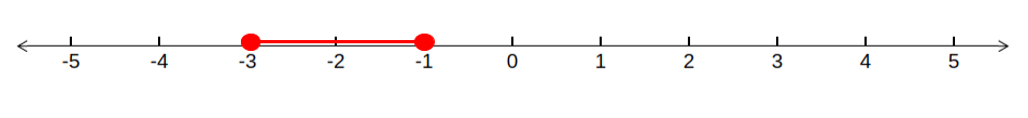
or in interval notation, the solution is : [-3,-1]

Let’s work through an example together¶

std_form1 = "-4x^2+8x+96<=0"

display(Latex('1.Consider the inequality $(-x)(4x - 8) \leq -96$.'))
display(Latex(' Re-write the inequality in standard form (use the symbol ^ to indicate an exponent and <= for the inequality sign).'))

inpt1 = widgets.Text(placeholder='Enter inequality')
text_warning1 = widgets.HTML()
button_check1 = widgets.Button(description="Check Answer")

display(widgets.HBox([inpt1,button_check1]))

def check_button1(x):
    inpt1.value = inpt1.value.replace(" ","")
    if inpt1.value==std_form1 :
        text_warning1.value="Very good!"
    else:
        text_warning1.value="Not quite - please try again!"

button_check1.on_click(check_button1)

display(text_warning1)

1.Consider the inequality: \[(-x)(4x - 8) \leq -96.\]

Re-write the inequality in standard form (use the symbol ^ to indicate an exponent and <= for the inequality sign.)

std_form2 = "x^2-2x-24>=0"
display(Latex('2.Consider the inequality we obtained in the first step.'))#: $-4x^2+8x+96\leq0$'))
display(Latex('We can simplify this further by reducing the leading coefficient to 1.'))
display(Latex('This can be done by simply dividing both sides by $-4$. If we do this, what does our expression become?'))

inpt2 = widgets.Text(placeholder='Enter inequality')
text_warning2 = widgets.HTML()
button_check2 = widgets.Button(description="Check Answer")

display(widgets.HBox([inpt2,button_check2]))

def check_button2(x):
    inpt2.value = inpt2.value.replace(" ","")
    if inpt2.value==std_form2 :
        text_warning2.value="Very good!"
    else:
        text_warning2.value="Almost! It's important to remember that if we divide or multiply an inequality by a negative number, we flip the inequality sign."

button_check2.on_click(check_button2)

display(text_warning2)

2.Consider the inequality we obtained in the first step.

We can simplify this further by reducing the leading coefficient to 1.

This can be done by simply dividing both sides by -4. If we do this, what does our expression become?

std_form3_1 = '(x-6)(x+4)>=0'
std_form3_2 = '(x+4)(x-6)>=0'
display(Latex('3.The next step is to factor our simplified polynomial expression.')) #: $x^2 - 2x - 24 \geq 0$.'))
display(Latex('Input the factored expression below:'))

inpt3 = widgets.Text(placeholder='Enter inequality')
text_warning3 = widgets.HTML()
button_check3 = widgets.Button(description="Check Answer")

display(widgets.HBox([inpt3,button_check3]))

def check_button3(x):
    inpt3.value = inpt3.value.replace(" ","")
    if inpt3.value==std_form3_1 or inpt3.value==std_form3_2:
        text_warning3.value="Correct!"
    else:
        text_warning3.value="Not quite - please try again!"

button_check3.on_click(check_button3)

display(text_warning3)

3.The next step is to factor our simplified polynomial expression.

Input the factored expression below:

display(Latex('Since we have $(x-6)(x+4)\geq 0$, there are the two sign possibilities; either'))
display(Latex('$1. ~ (x-6)\geq 0$ and $(x+4)\geq 0$'))
display(Latex('or'))
display(Latex('$2. ~ (x-6)\leq 0$ and $(x+4)\leq 0$'))

Since we have \( (x-6)(x+4)\geq 0\), there are the two sign possibilities; either

\[1. ~ (x-6)\geq 0 \text{ and } (x+4)\geq 0\]

\[or\]

\[2. ~ (x-6)\leq 0 \text{ and } (x+4)\leq 0\]

std_form4 = 'x>=6'

display(Latex('4. Consider expression $1.$'))
display(Latex(' Can you see what solution satisfies both $(x-6)\geq 0$ and $(x+4)\geq 0$? Enter your answer below in the form "x>= _"'))

inpt4 = widgets.Text(placeholder='Enter interval')
text_warning4 = widgets.HTML()
button_check4 = widgets.Button(description="Check Answer")

display(widgets.HBox([inpt4,button_check4]))

def check_button4(x):
    inpt4.value = inpt4.value.replace(" ","")
    if inpt4.value==std_form4 :
        text_warning4.value="Very good! Since we are looking for values of x that are larger than 6 and -4, and 6>-4, the first expresssion gives us one simple solution interval: x>=6"
    else:
        text_warning4.value="Not quite - please try again!"

button_check4.on_click(check_button4)

display(text_warning4)

4. Consider expression 1.

Can you see what solution satisfies both \((x-6)\geq 0\) and \((x+4)\geq 0\)? Enter your answer below in the form "x>="

std_form5 = 'x<=-4'

display(Latex('5.Now consider expression $2$ What is the interval satsfying these inequalities?'))

inpt5 = widgets.Text(placeholder='Enter interval')
text_warning5 = widgets.HTML()
button_check5 = widgets.Button(description="Check Answer")

display(widgets.HBox([inpt5,button_check5]))

def check_button5(x):
    inpt5.value = inpt5.value.replace(" ","")
    if inpt5.value==std_form5 :
        text_warning5.value="Very good! Since we are looking for values of x that are less than -4 and 6 and 6>-4, this expresssion also gives us one simple solution interval: x<=-4"
    else:
        text_warning5.value="Not quite - please try again!"

button_check5.on_click(check_button5)

display(text_warning5)

5.Now consider expression 2 What is the interval satsfying these inequalities?

std_form6 = '(-inf,-4]U[6,inf)'

display(Latex('6. So, what is our final solution interval for the inequality $(-x)(4x - 8) \leq -96$?'))
display(Latex("Enter your answer in interval notation, using the following notations if necessary: 'U' for union symbol and 'inf' for infinity"))
inpt6 = widgets.Text(placeholder='Enter interval')
text_warning6 = widgets.HTML()
button_check6 = widgets.Button(description="Check Answer")

display(widgets.HBox([inpt6,button_check6]))

def check_button6(x):
    inpt6.value = inpt6.value.replace(" ","")
    if inpt6.value==std_form6 :
        text_warning6.value="Excellent! Now let's see how the solution looks like on the number line"
    else:
        text_warning6.value="Not quite - please try again!"

button_check6.on_click(check_button6)

display(text_warning6)

6. So, what is our final solution interval for the inequality \((-x)(4x - 8) \leq -96\)

Enter your answer in interval notation, using the following notations if necessary: 'U' for union symbol and 'inf' for infinity

button7 = widgets.Button(description="Display solution on  a number line",layout=Layout(width='40%', height='50px'))

display(button7)

def display_button7(x):
        img = mpimg.imread('images/ex_soln.png')
        fig, ax = plt.subplots(figsize=(18, 3))
        imgplot = ax.imshow(img,  aspect='auto')
        ax.axis('off')
        plt.show()
        button7.disabled=True

button7.on_click(display_button7)

Callysto Curriculum Notebooks

Intervals and inequalities¶

Polynomials¶

Intervals of Inequalities¶

Interval Notation¶

Solving Inequalities¶

Let’s work through an example together¶

Graphical visualization of inequality solutions¶

Changing Parameters¶

Constant term¶

Extra Problems¶

Practice solving graphically¶

Solve the inequalities¶

Plotting in Python¶

Conclusion¶